Fast Robots: ECE 4960 Lab 12
Objective
In this lab, I will continue to make the robot perform high-speed wall following along an interior corner. I plan to add a Kalman Filter to estimate the full state before applying the LQR controller to improve the robot’s performance. The goal of the lab is to hit the corner full speed and still move along the second wall after turning.Tune the Kalman Filter
From the lab 11 results, I noticed that the theta and the proximity distance would have a larger error while the timestamp increased. Therefore, to improve the LQR controller, I decided to use a Kalman Filter to estimate the full state by giving limited measurements (proximity and thetadot). After I got the estimated full state of the robot, I will take the estimation into the LQR controller to get the proper force, so the robot can be controlled much better. I followed the instructions from the lecture to implement a Kalman Filter in Matlab. The overall program is shown in Figure 1.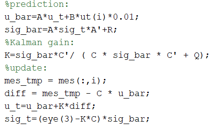
Figure 1. The Kalman Filter program in Matlab.
To tune the Kalman Filter, I used the data from Lab 11 and observed how the filter worked by testing with different parameters which are the process noise (R), measurement noise (Q), and force (ut). The dimension of the process noise (R) and the dimension of measurement noise (Q) should be 3 by 3 matrices. From the results, it seems that the fluctuation is smaller and smoother while the process measurement (R) is larger. This did match my expectations because the prediction covariance (sig_bar) will be affected by the noise. Besides, I noticed that when the measurement noise (Q) is larger, the system will trust the prediction position more because the Kalman gain will be smaller. The final value for R and Q I used is shown in parameter Figure 2. I decided on these values from the testing and the data observation from the measurements. Besides, I scaled down the force to 0.1 of the original to make the filter work. I think the factor was related to the sample rate I used to collect the data. The result is shown in Figure 3.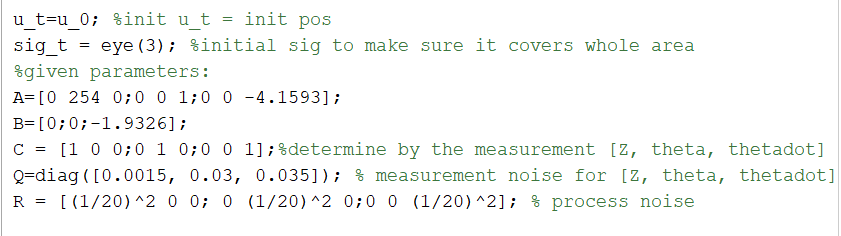
Figure 2. The parameters of KF.
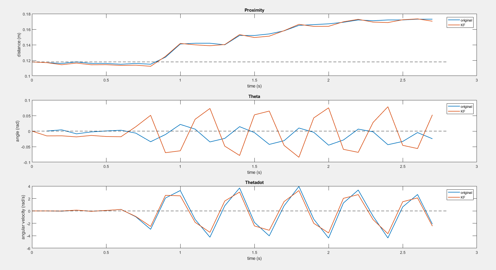
Figure 3. The KF on the lab 11 data.
LQG Wall Following
Once I completed the Kalman Filter tunning, I implemented the same code on the actual robot and modified the current state in the find_force function. Both functions are shown in Figure 4. Then, I tested the robot and plotted the result in Figure 5.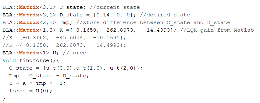
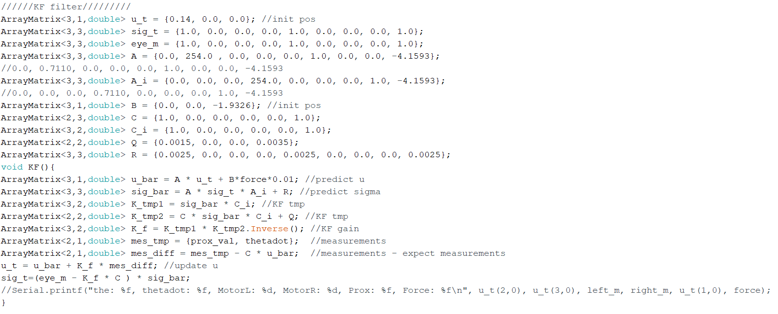
Figure 4. The find_force function (left) and the KF function (right).
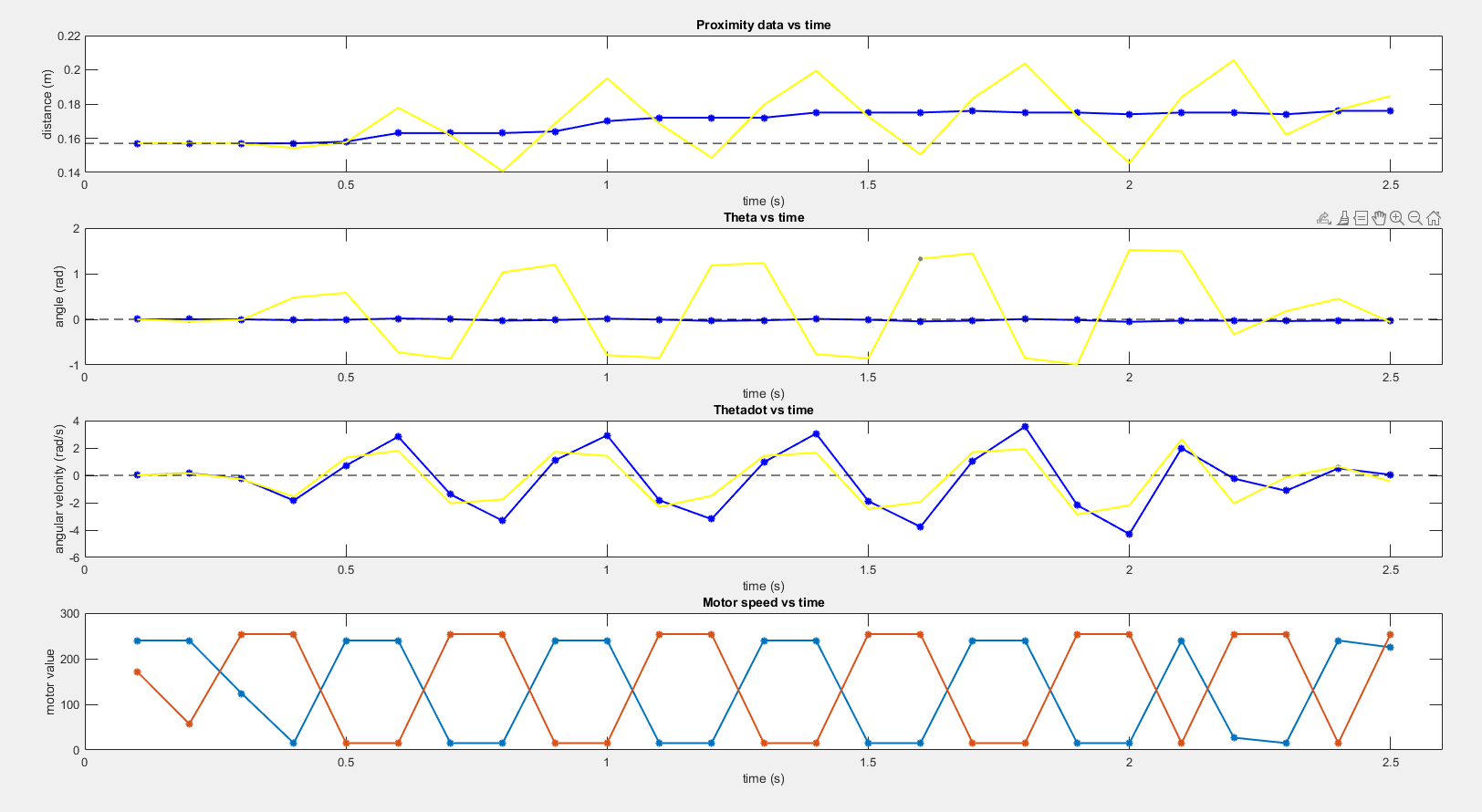
Figure 5. The LQR with KF result. (Blue: raw state, Yellow: estimated state)
According to the diagram, I noticed that the estimated state was quite large than the raw state, so I tried to debug it on Matlab. Then, I realized that I changed the sample rate to 0.01 sec per data, so the force should be multiplied by 0.01. The comparison data is shown in Figure 6.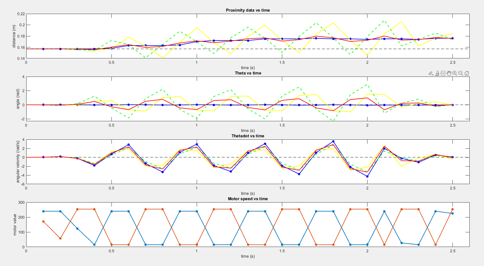
Figure 6. The comparison data of LQR with KF. (Blue: raw state, Yellow: estimated state, Green: Matlab estimated state, Red:fixed estimated state)
After that, I ran the second test with the LQR and KF to verify everything worked well. From the result in Figure 7, I believed that the program and the robot worked well. Besides, the comparison of the process with KF and without KF shows in Video 1, and the robot with KF was more stable than the robot without KF.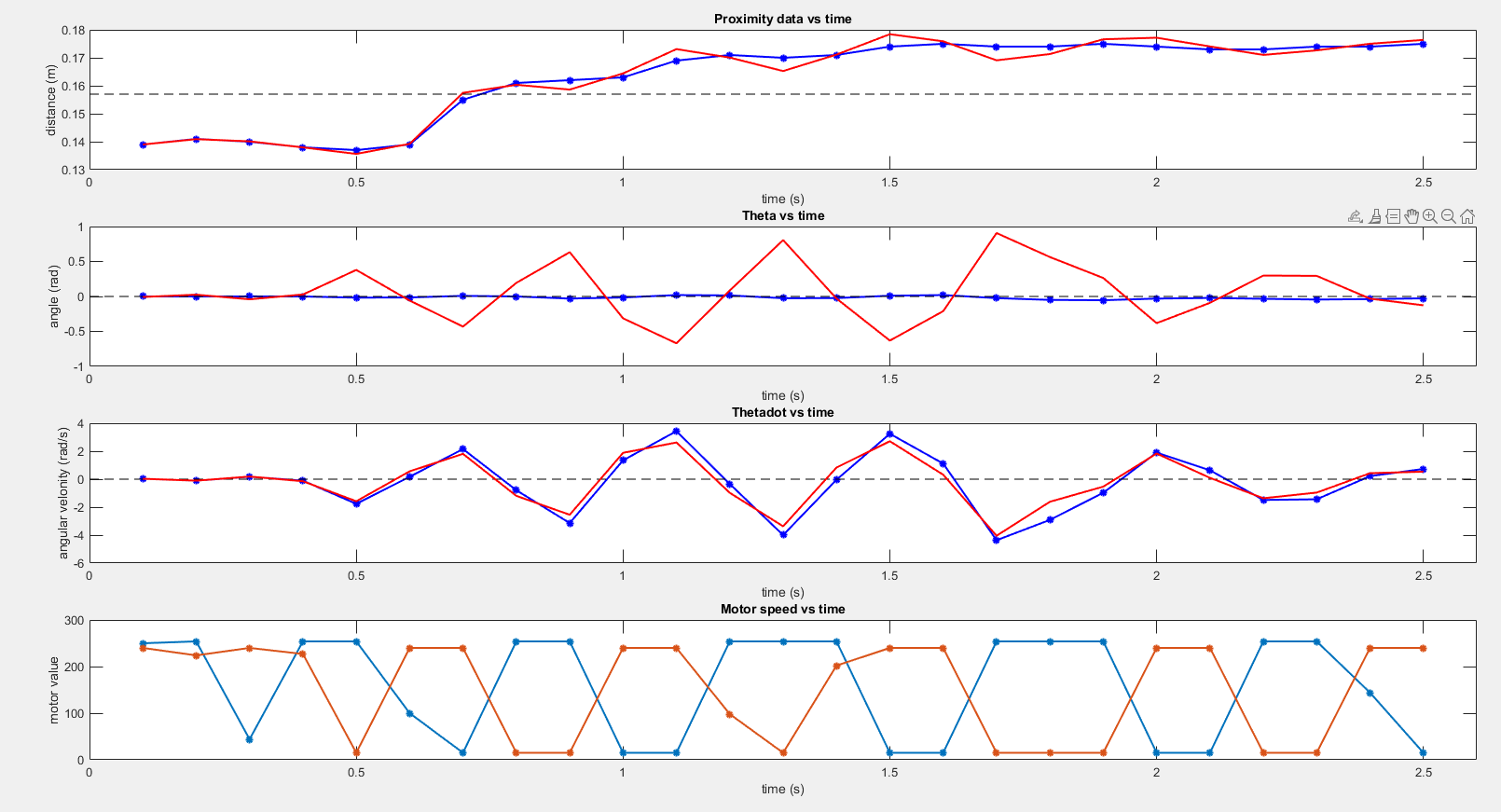
Figure 7. The success LQR with KF data.(Blue: raw state, Red: estimated state)
Video 1. The comparison of the LQR without KF (left) and LQR with KF (right).
Turn the Corner
Next, I implemented the robot to turn 90 degrees when it sees the wall. Before writing the code, I tested the theta value from gyroscope Z reading and noticed that the value will be around -0.1 when the robot turned 90 degrees. Therefore, I made a conditional statement to make the robot turn when the TOF sensor was smaller than 0.38 meters. I got the “0.38” value by doing several tests and this threshold value has larger repeatability. The robot will stop turning if either the theta value is smaller than -0.1 or the turning cycle is greater than 3. Again, I got the threshold from experiments. Moreover, I lower the maximum motor value to 200 and 190 for left and right motors respectively to have better performance. In Video 2, the robot can successfully turn when it saw a wall.Video 2: The turning process demonstration.
Re-engage LQR
Last, I re-engaged the LQR controller with KF on the robot after the turn. The main function I operated is shown in Figure 8. I found that the robot would be hard to move straight, so I changed the gain of the LQR controller to penalized the proximity distance more and the new gain is shown in Figure 9.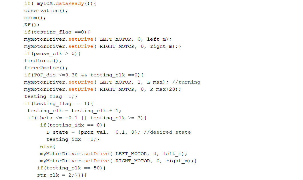
Figure 8. The main function of the robot.
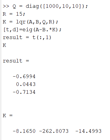
Figure 9. The gain of the LQR.
After running the robot with the new LQR gain, the robot could successfully turn and follow the second wall, which shows in Video 3. It was important to reset the setpoint for theta as the car has turned 90 degrees. I used the value -0.1 for theta setpoint which I mentioned in the previous section and the first proximity value after turning for the distance setpoint in the new desire state. The raw state and the estimation state results are shown in Figure 10.Video 3. The LQR engaging after turning the robot.
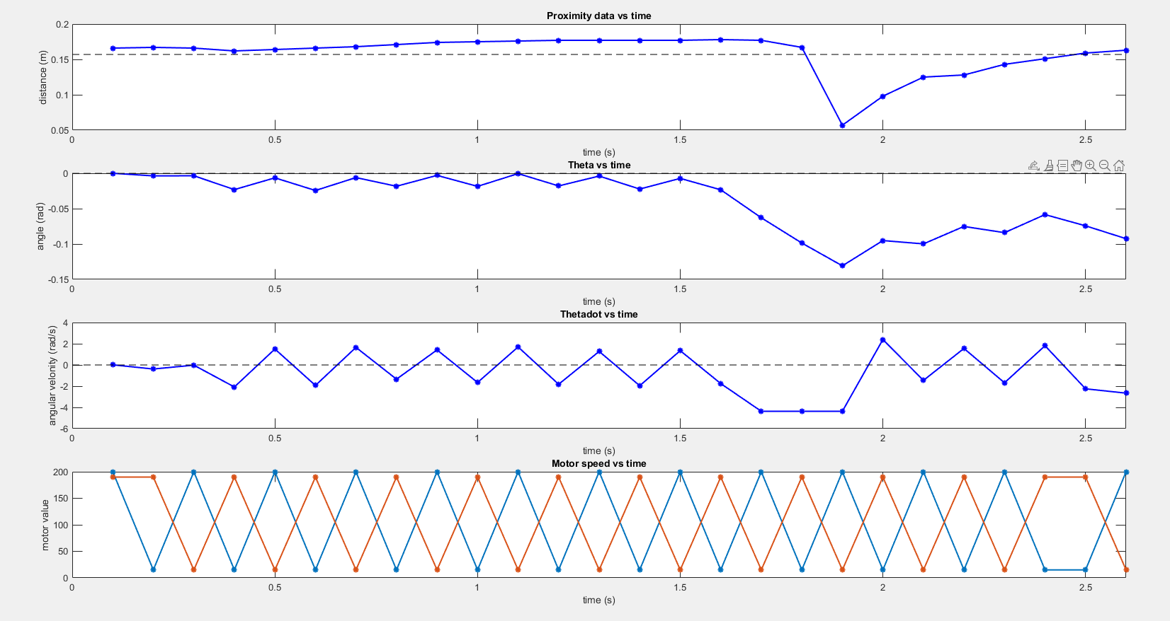
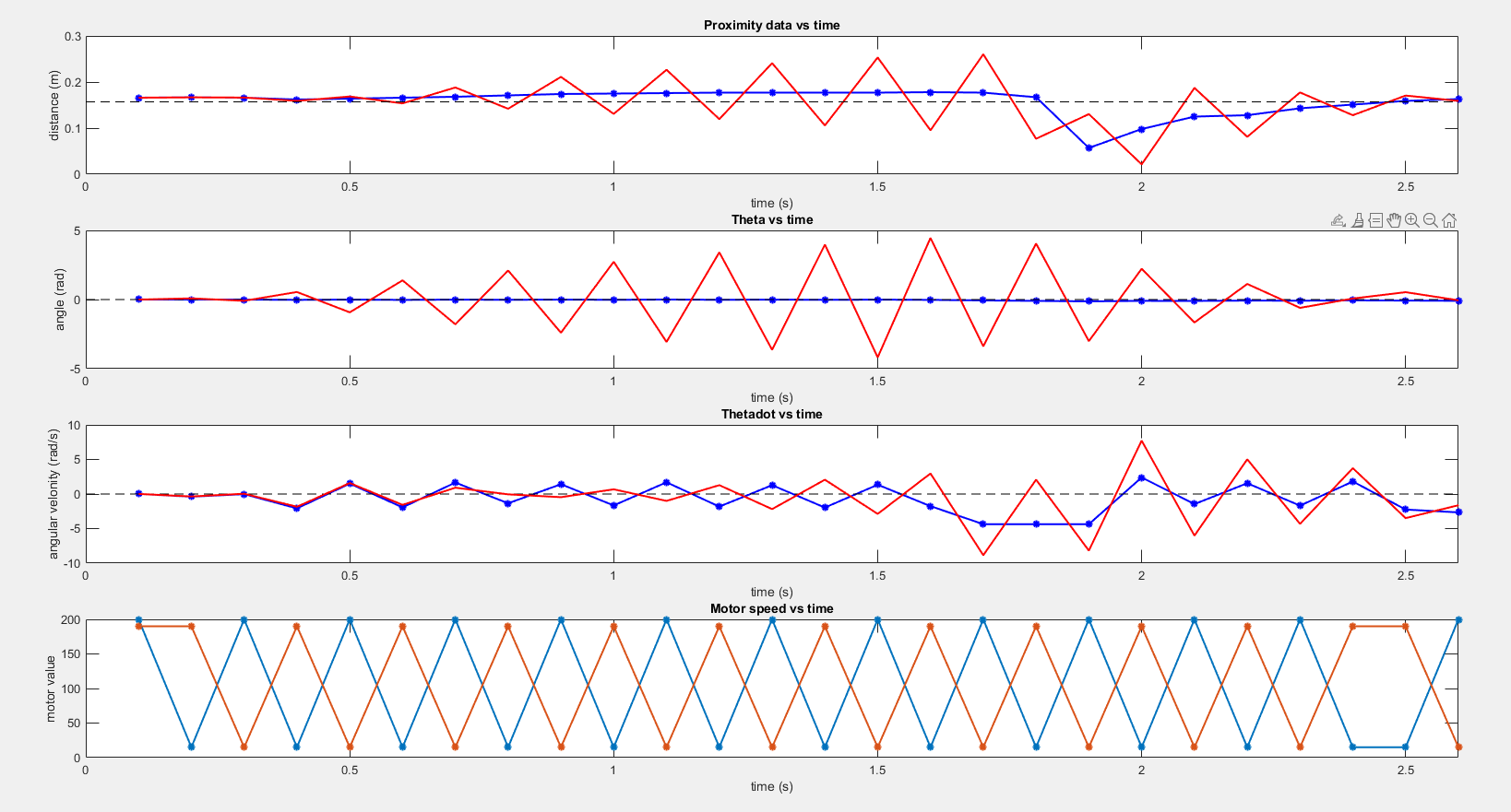
Figure 10. The robot states result in theta setpoint = -0.1.: Raw state (top) and Comparison result (bottom).
[Blue: raw state, Red: estimated state]
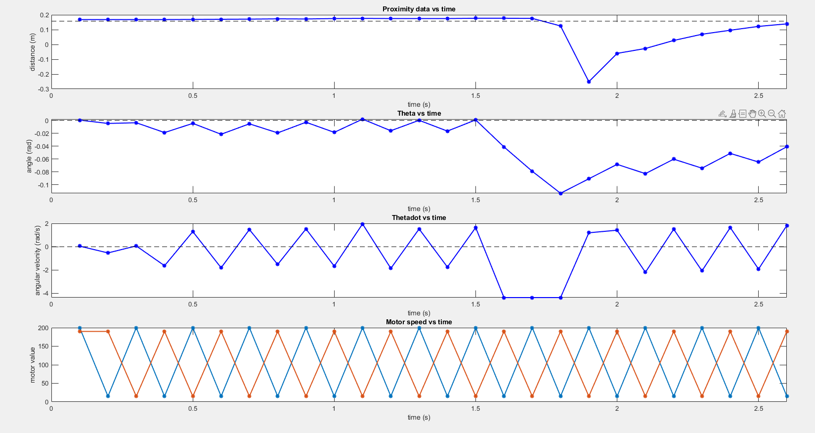
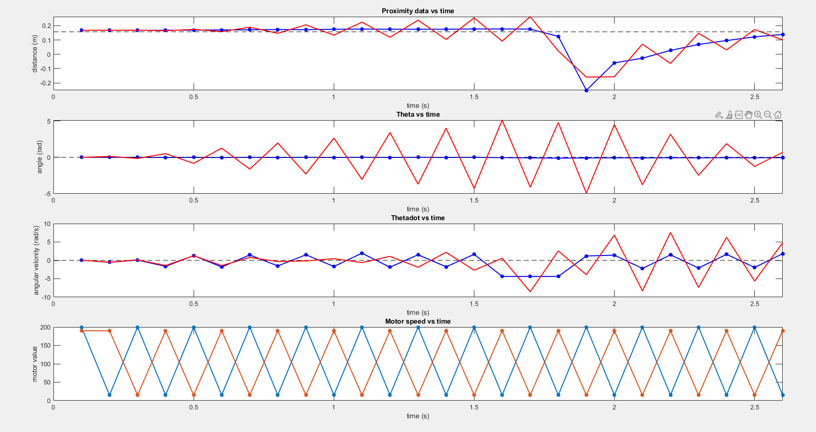
Figure 11. The robot states result in theta setpoint = -0.05.: Raw state (top) and Comparison result (bottom).
[Blue: raw state, Red: estimated state]
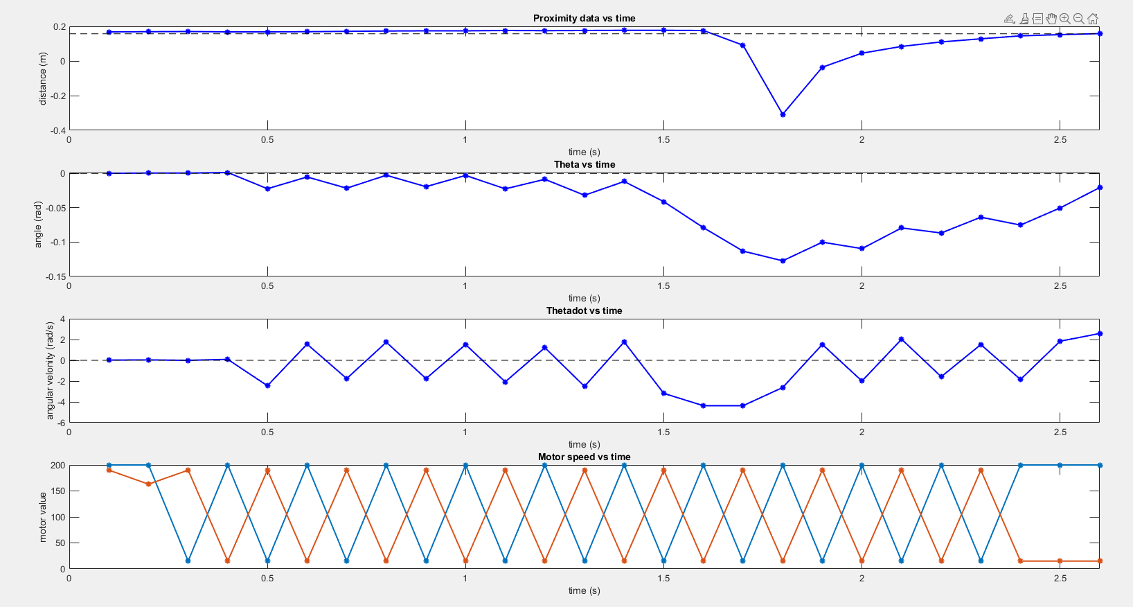
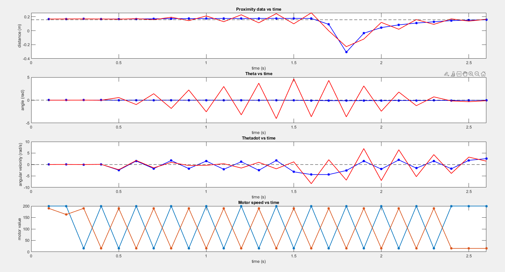
Figure 12. The robot states result in theta setpoint = 0.: Raw state (top) and Comparison result (bottom).
[Blue: raw state, Red: estimated state]