Fast Robots: ECE 4960 Lab 7
Objective
From the last lab, I have compared the truth pose estimation and odometry estimation and realized that the odometry trajectory had huge errors, so it is important to apply the filter on the odometry data to get a better localize estimation. The purpose of this lab is to prepare the precursor program for the next lab which will implement grid localization using Bayes Filter. Also, this lab will ask the students to create an environment and map it with the robot’s sensors for future localization experiments.Lab 7(a): Grid Localization using Bayes Filter
I downloaded the lab 7 distribution code and played around with the program. I ran the robot without any filter or control implementation and plotted the robot’s truth pose and its odometry trajectory. Figure 1 shows the odometry trajectory has a large offset of the truth pose, which is the same result I got in lab 6.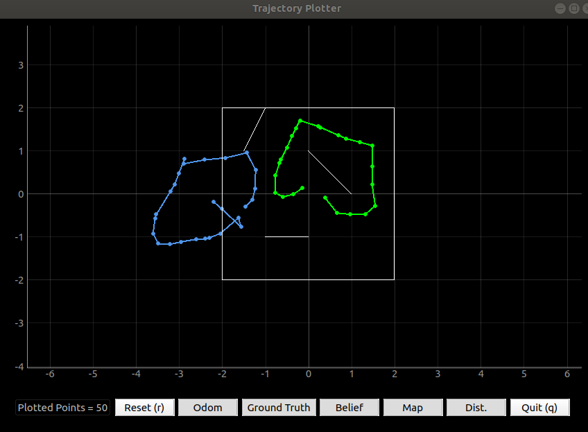
Figure 1: The comparison of odometry and truth pose.
Video 1: The plotting progresses while the robot is moving.
Therefore, I started following the instructions to complete the precursor program. The first step was to write the computation control function. I read the class slide and the robot motion paper to calculate the rotation and the transition from the odometry data.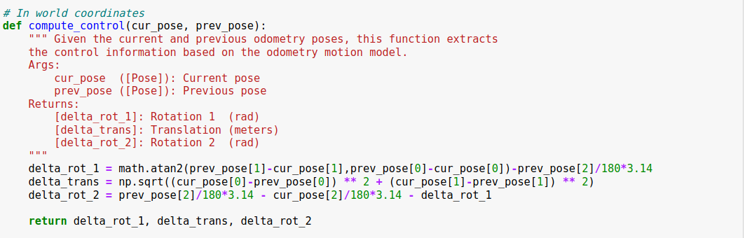
Figure 2: The code of the compute control program
Next, I wrote the odometry motion model function to calculate the probability of state transitionP(x’ | x, u) . This function will be used in the prediction step of the Bayes filter. It will take the Gaussian distribution for the three parameters (rotation 1, transition, and rotation 2) for all the possible locations.
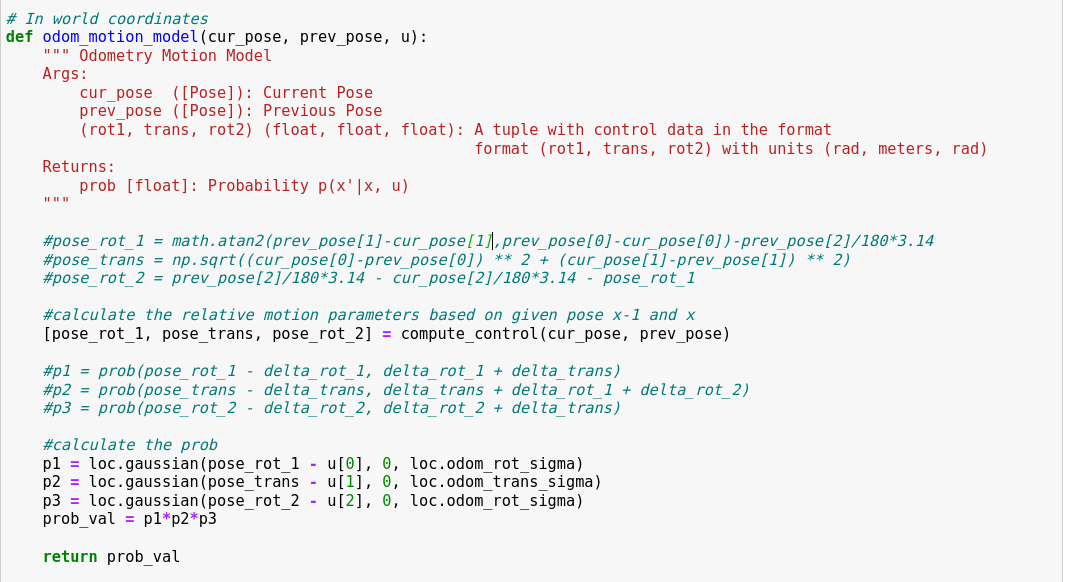
Figure 3: The code of the odometry motion model program.
The next step is to write the prediction step of the Bayes filter. This function is used to update the belief bar based on the belief from the previous time step and the odometry motion. The function will find the belief of the previous position and compare it with all the possible grid in order to find the probability of the new position. Therefore, it will need to take 51 million loops to finish the calculation for all the grid. So, I tried to consider the grids that have the value of beleif to do the calculation and the rest belief bar will still be zero becuase the previous belief was zero. In this case, it can take about 7200 times cycle to complete the prediction process. It is much faster.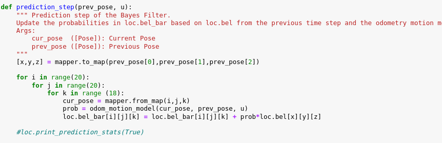
Figure 4: The code of the prediction step.
Then, I wrote the sensor model function to calculate the probability of the measurementP(z | x) for the update process. The function will calculate the Gaussian distribution from the sensor measurement and the expected measurement that was provided from the course.
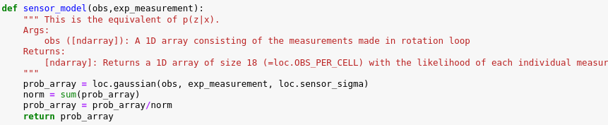
Figure 5: The code of the sensor model.
Last, I finished the update step of the Bayes filter. In this step, the function will take the measurement data with the expected measurement value into the sensor model function to find the probability of each grid. Besides, It is important to normalize the probability to allows us to get the probability for the occurrence of an event, rather than merely the relative likelihood of that event compared to another.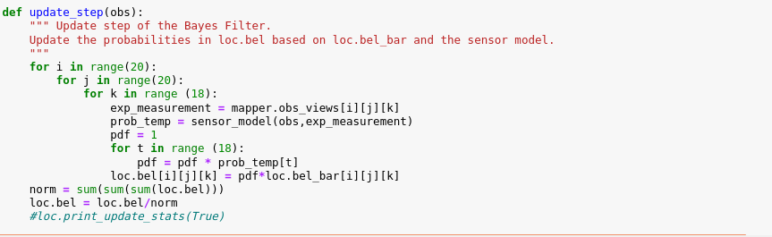
Figure 6: The code of the update step of the Bayes filter.
Once I finished the precursor program, I was curious whether the program works properly. Therefore, I tried to implement the program when the robot went linearly. Video 2 shows the process of the odometry assumption with the Bayes filter. Although the first assumption point was far away from the true point, I believed that my function worked properly because the initial distribution was zero for all the grids except the initial point. Therefore, there was may possible location which had a similar expected measurement if the environment symmetry, so it was hard to find the real point of the robot. However, the odometry trajectory was eventually converged to the truth pose trajectory, so I believe that my code works properly.Video 2: The demonstration of the Bayes filter with the linear motion.
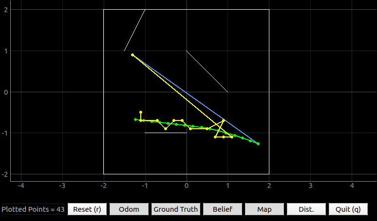
Figure 7: The trajectory between the belief and the truth poses with the linear motion.
Moreover, I tried the robot with the motion control that was given by the distribution code, which will go straight and rotate per cycle. The Bayes filter works properly as well. So, I will do more tests and discuss more results in the next lab.Video 3: The demonstration of the Bayes filter with the dynamics motion.
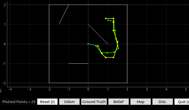
Figure 8: The trajectory between the belief and the truth poses with the dynamics motion.
Lab 7(b): Mapping
In this section, I am going to set up an environment for robot localization in the future lab. I have set up a room whose dimensions are 2.75 m x 1.5 m. To make it interesting, I placed two boxes in the middle of the room to pretend like the islands. The overview of the environment is shown in Figure 9.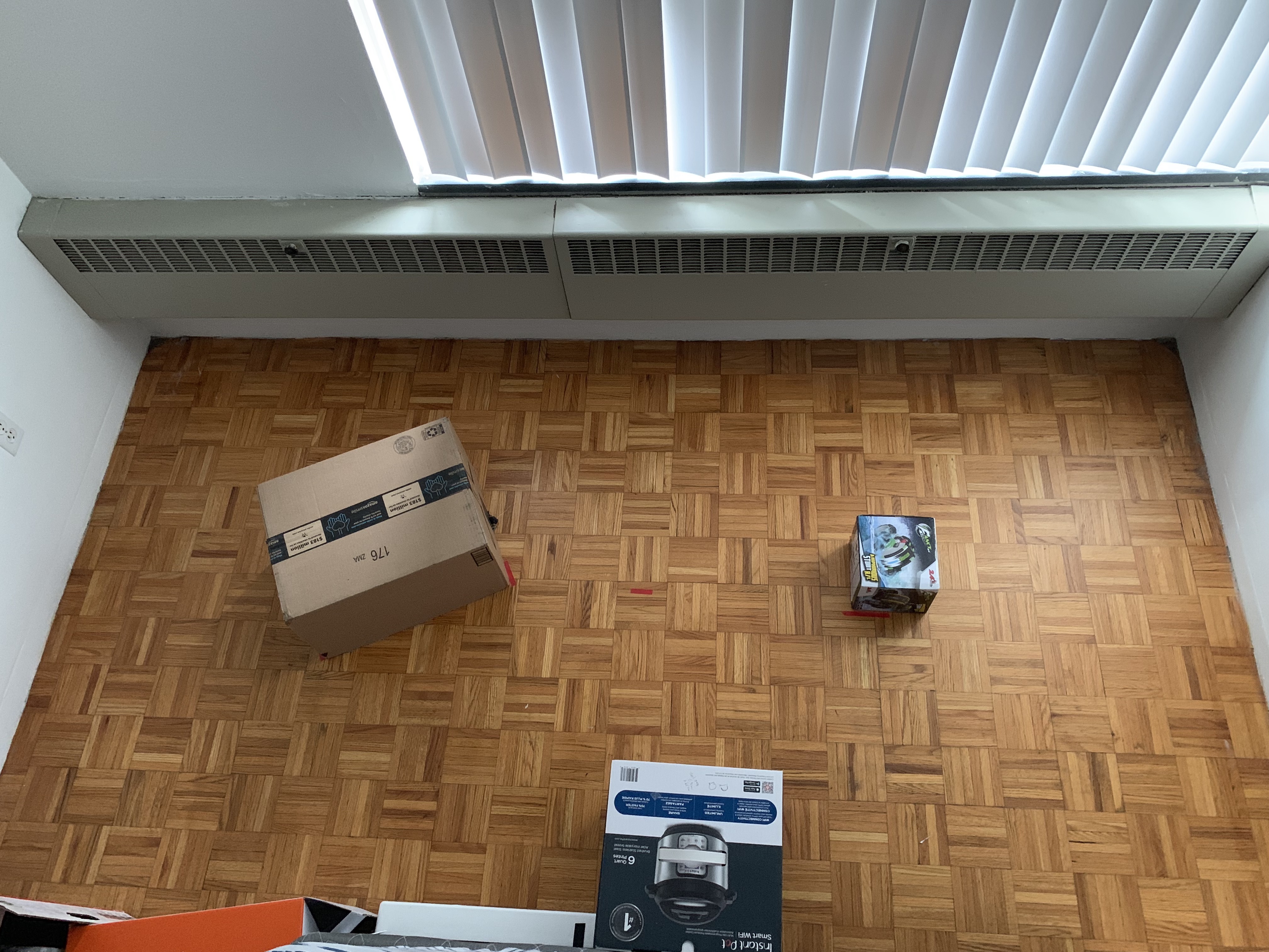
Figure 9: The overview of the room environment.
Before I started mapping, I made a sanity check by placing the robot at the corner and rotating the robot to scan the environment. I collected the TOF distance measurements and the yaw value from the IMU sensor to generate the line diagram and the polar plot. I compared the data with the real environment which shows in Figure 10. The data seems reliable to me.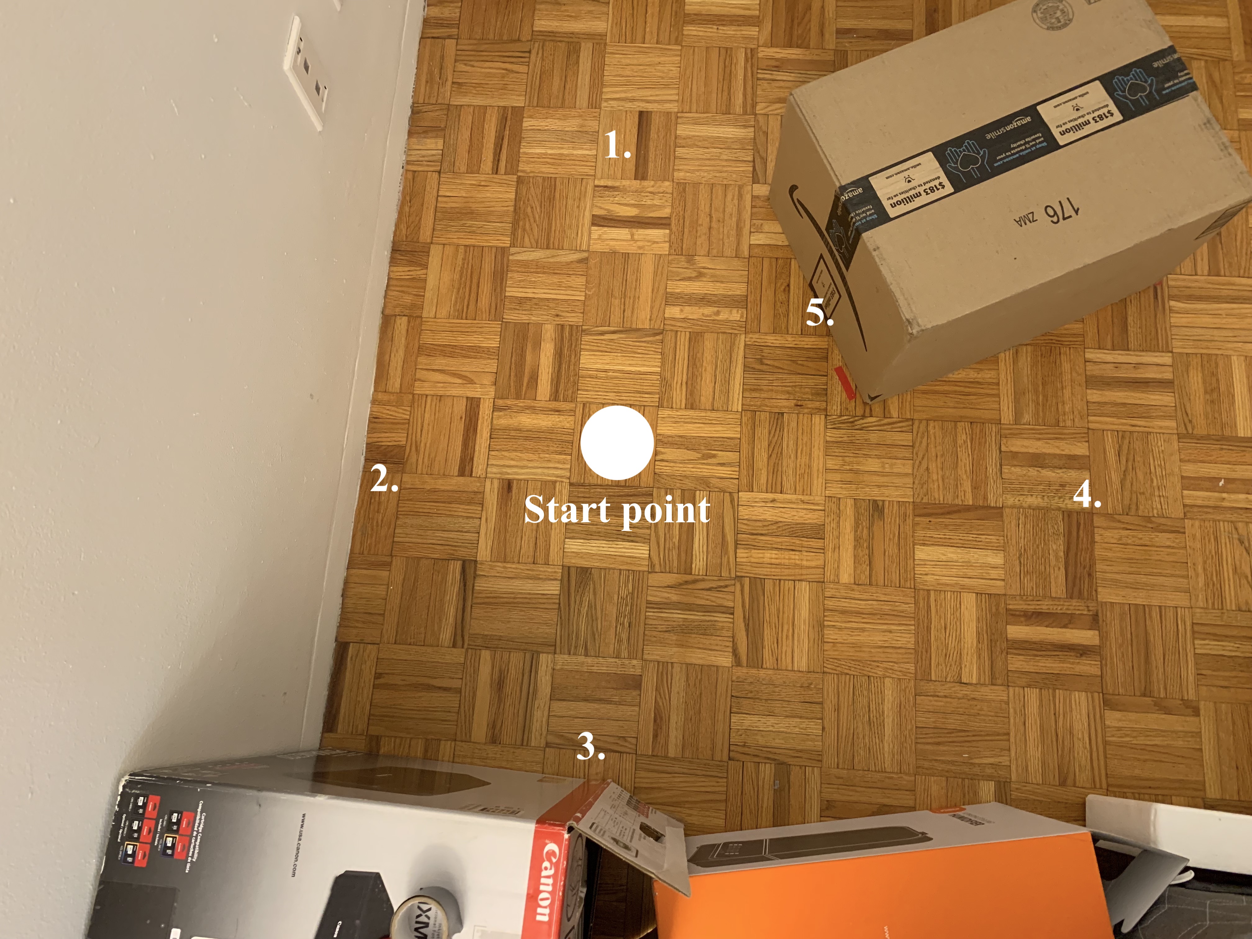
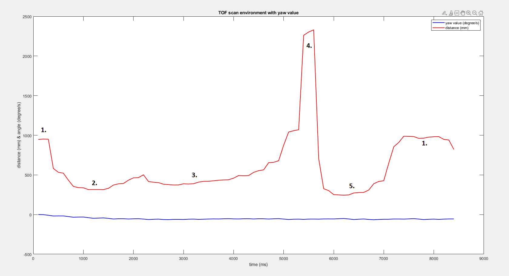
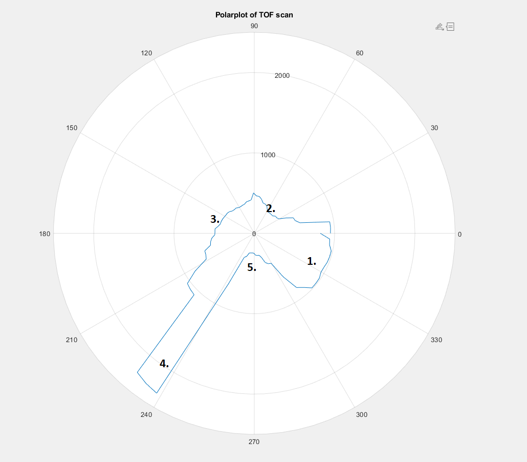
Figure 10. The real environment (left), the line diagram of the data (middle), and the polar plot (left).
Besides, I have made the tests three times in order to see how reliable the data is and determine the repeatability of the measurements. In Figure 11, it shows the comparison between these three tests. I saw the yaw value was almost the same and the pattern of these tests looked similar, but the time of the measurements was slightly different. I believed the reason was the speed of the motor that controlled by the PID controller which makes the angle increments different.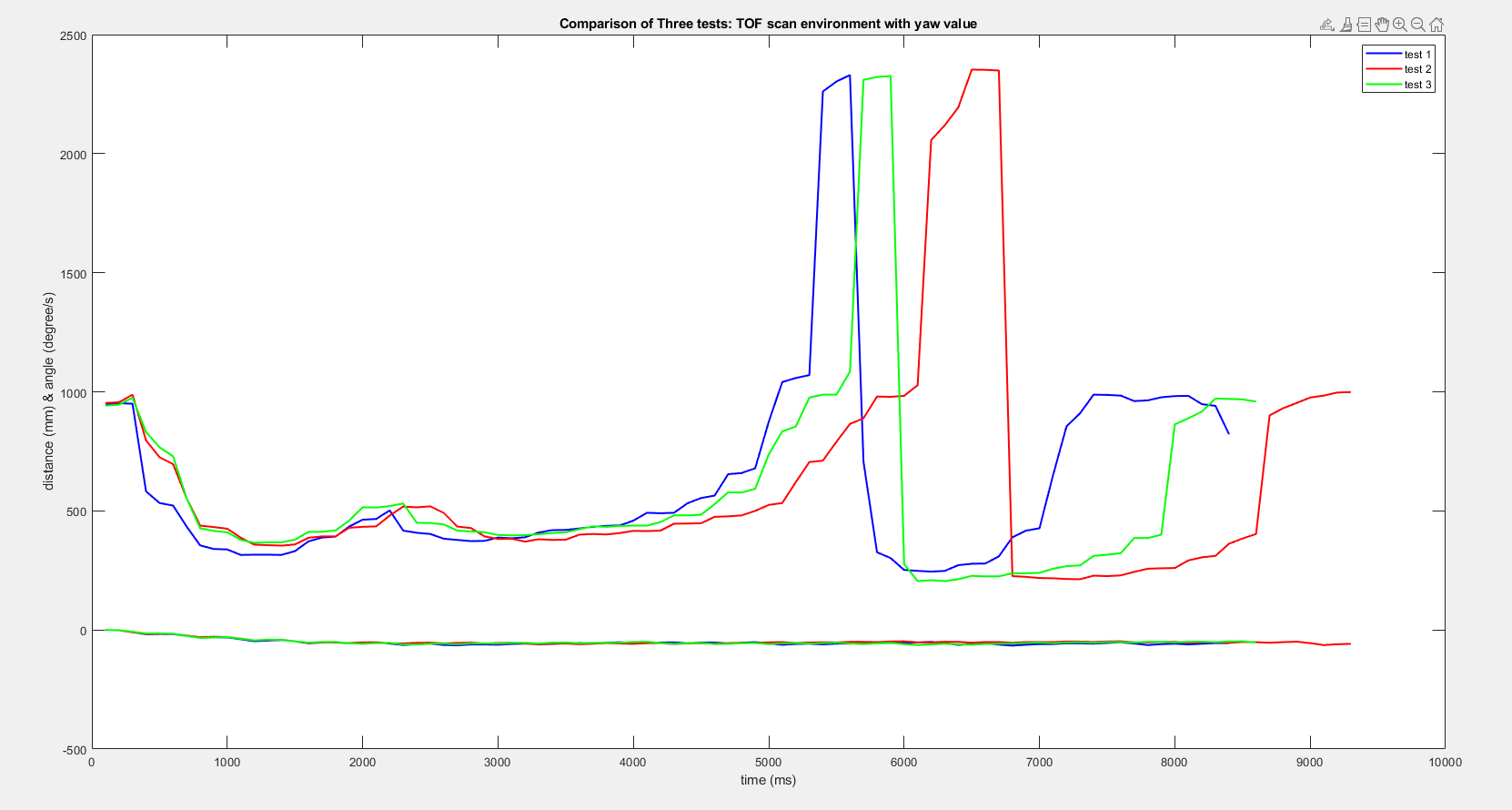
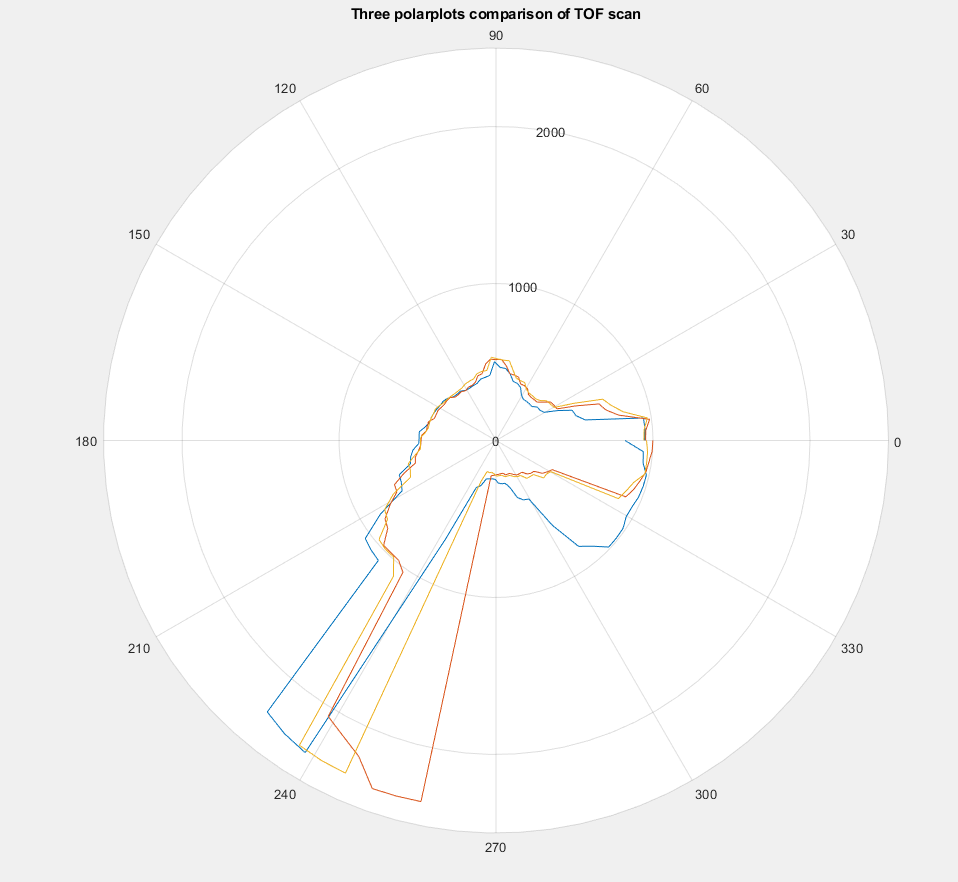
Figure 11: The comparison data of three different tests.
Next, I checked the coordinates of each sensor to ensure the measurements could be converted to the inertial reference frame of the room. Both the proximity sensor and TOF sensors had the same coordinates of the room, but the IMU sensor had a different frame. I drew the frame and showed the transformation matrices that I used in Figure 12.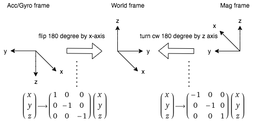
Figure 12: The IMU frame with the transformation matrices.
After I finished the sanity check, I built the map manually. I placed the robot in known poses and performed line scans. I collected all the data and used Matlab to make a scatter plot and connected the room boundary with lines, which shows in Figure 13.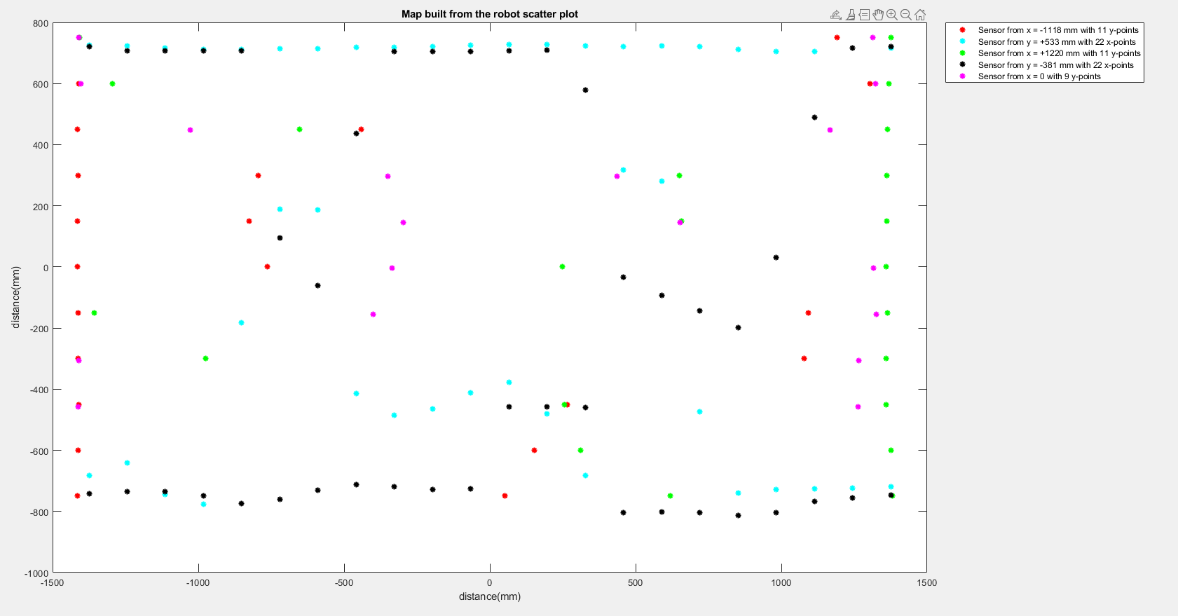
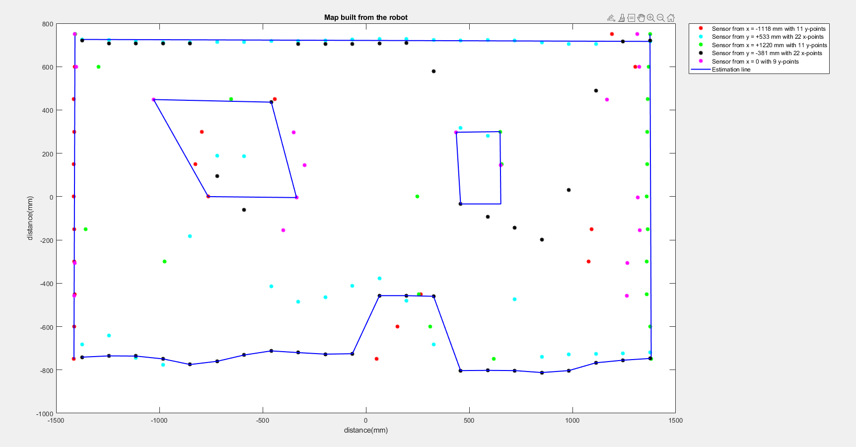
Figure 13: The scatter plot and room estimation.
Moreover, I analyzed the yaw value and calculated the robot rotation time. I found the robot will rotate 50 degrees per second, so it will take 7.2 seconds to complete a 360-degree rotation. In order to pair the measurements with 18 readings of the simulator, I will need 0.4 seconds to collect data and each cycle of the code took 130 ms, so I made the program to collect the data every four cycles. The other code was the same as the code that I used in lab 6.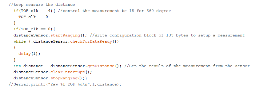
Figure 14: The code of control the TOF measurements.
Last, I wrote a room boundary list in order to visualize your map in the plotter tool of the simulator. The list is shown in Figure 15 and the map is shown in Figure 16.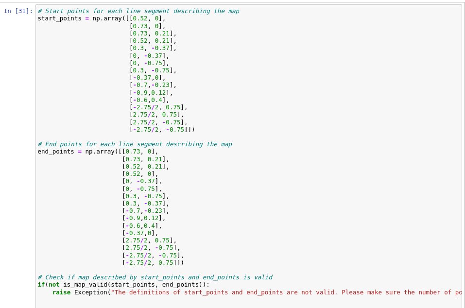
Figure 15: The start points and end points list.
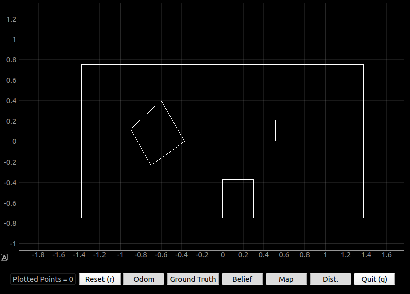
Figure 16: The map in the plotter tool of the simulator.