Fast Robots: ECE 4960 Lab 9
Objective
The purpose of this lab is to implement the Bayes filter on the actual robot and try to localize the estimated position. The course has provided a fully-functional and optimized Bayes filter implementation that works on the virtual robot. I will modify the code and make the module be able to communicate with the real robot through Bluetooth. Then, I will run several tests and compare the difference from the simulations to the practical results.Implementation
Before starting the implementation, I need to set up the environment for the testing. The procedure has done in Lab7(b). After the testing environment has set up, I started working on the Bluetooth program that I wrote in Lab 2. I needed to send three odometry information (x-odom, y-odom, and yaw) and 18 distance measurements to the base station. Because the total number of the data is 21, I added six additional float variables into the function, so the program would be able to send seven data at the same time. I will just need three cycles to get the data for one interaction of the Bayes filter process. The code is shown in Figure 2. The program worked properly for sending a constant value, so I continued to the next step.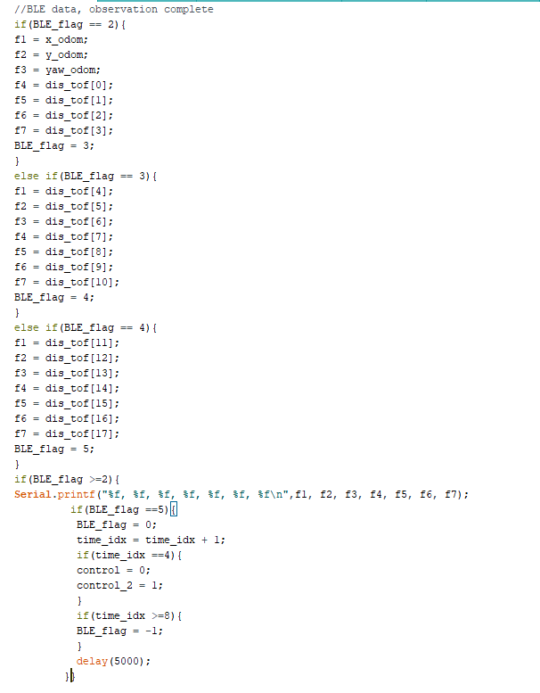
Figure 1: The Bluetooth data module.
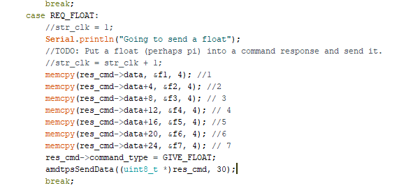
Figure 2: The Bluetooth request_float function.
Then, I started thinking about how my code could control the robot to move between each interaction of the Bayes filter. I took the suggestion from the guideline, but instead of sending the motion commands from the base station to the robot, I stored the different time for each interaction inside the robot at a constant speed. The reason I did not send the control command through Bluetooth was that the wireless communication was unstable on my program and my computer kept freezing while I ran too many commands through Bluetooth, so I would like to make the wireless program be simple. Therefore, I wanted to make my robot to move an 8 shape, so I measured the distance for the eight expected locations and tested the speed with each time difference to find the ideal number for each interaction. In Video 1, it shows that how I adjusted the time for each interaction. Besides, I measured the time of 360-degree rotation which was about 3 seconds, so I used a while loop with a 0.15 seconds time delay to get the 18 equally spaced measurements from the TOF sensor. The completed program is shown in Figure 3.Video 1: The demonstration of the robot sequence motion.
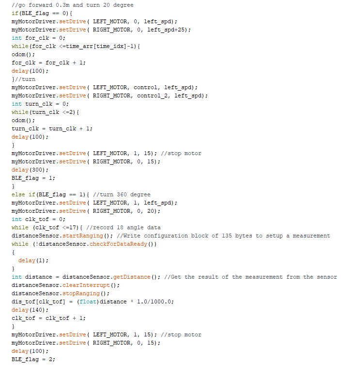
Figure 3: The motion control and TOF measurement program.
Next, I integrated the wireless program with the motion control program together. Once I ran the program, there were three situations occured randomly. First, the robot could run properly, but the PID controller would be very unstable, which led the TOF scan inaccurate. I believed that the reason was the wireless transmission time caused a delay and made the PID controller increased the speed in order to achieve the setpoint. To solve this problem, I thought I could write a multithread program to eliminate the delay for the PID controller. Second, the program cannot synchronize with the base station, so the data cannot be sent successfully. I could not find the reason why the float command cannot be received. The error message shows in Figure 4.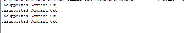
Figure 4: The error message shows “unsupported command”.
Third, the Bluetooth adapter would fail after the message that shows in Figure 5 poped out. I cannot find a reason for this issue either. The only solution I knew was to restart my computer twice, which was really time-consuming.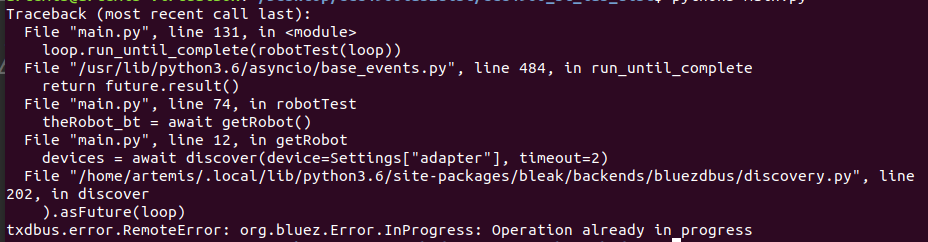
Figure 5: The error message that made the Bluetooth not work.
Moreover, I ran the wireless python program directly on the Jupyter notebook, and the program could run only one time. When I stopped the program, the Bluetooth passthrough of the VM would be interrupted. Although I unplugged and re-plugged the Bluetooth adapter, it would not solve the problem but make the Bluetooth fail directly.Solution
In order to complete the lab, I decided to run all the eight interactions with the USB cable and stored the data in a text file. Then, I wrote a Matlab function to create an array for each interaction, so I could copy and paste the dataset to the Jupyter notebook. Once I got the dataset, I could run the Bayes filter and compare the estimation with the truth pose. The main function is shown in Figure 6, the data function is shown in Figure 7, and the data sort function is shown in Figure 8.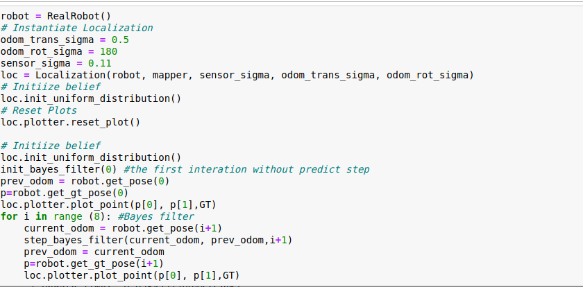
Figure 6: The main function of the Bayes filter.
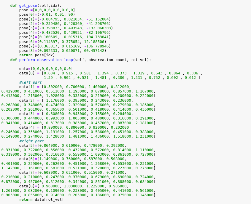
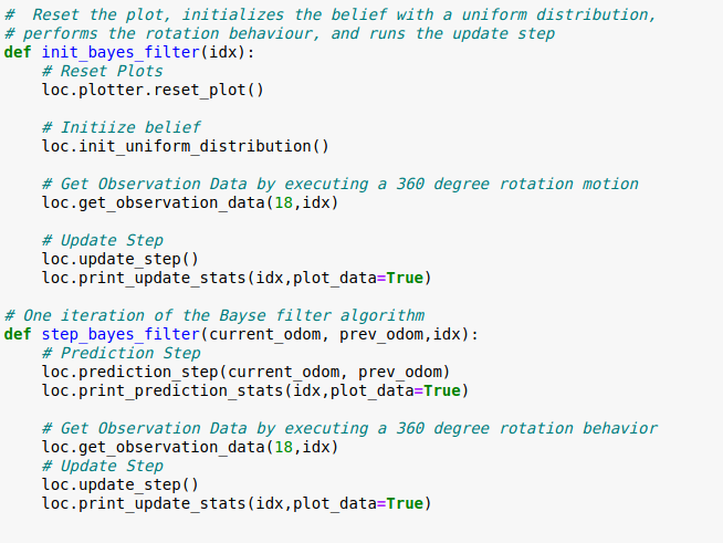
Figure 7: The data function for the Bayes filter.
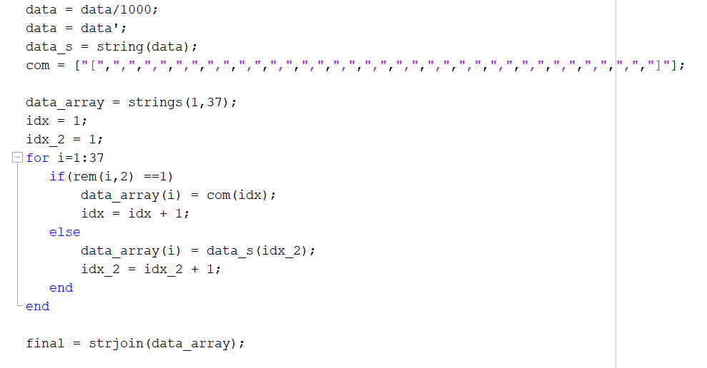
Figure 8: The data sort function in Matlab.
I made two flow-charts in Figure 9 to show the difference between the ideal implementation and my implementation. In my opinion, using Bluetooth will be more realistic and efficient for the test in the real world, but there is no huge difference and benefits between the results of these two methods, so I think that my solution could work properly.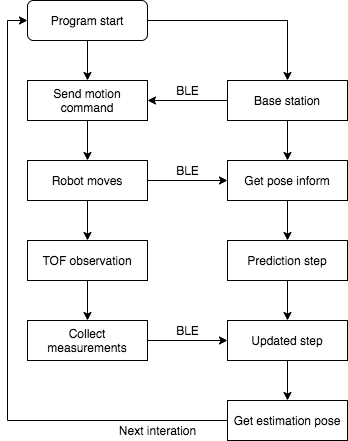
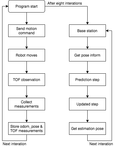
Figure 9: The flow-chart of the ideal implementation (left), The flow-chart of my implementation (right).
Result & discussion
Once I finished the code, I made two different experiments that are using a uniform prior to the pose with only the update step and testing a sequence motion with the Bayes filter. In the uniform experiment, I picked five points on the map and ran only the update step of the Bayes filter to observe the estimated position. The result is displayed in Figure 10. I noticed that the estimated position of tests 1, 3, and 4 was closed to the ground truth. Tests 2 and 5 had a huge deviation in the true position. The reason is that tests 1, 3, and 4 have more unique characteristics of the position, which means that the probabilityP(z | x) is more unique and relatively higher. The surrounding of Tests 2 and 5 are relatively empty and there are no recognizable objects nearby, so the TOF measurements are quite similar, which leads to the prediction errors.
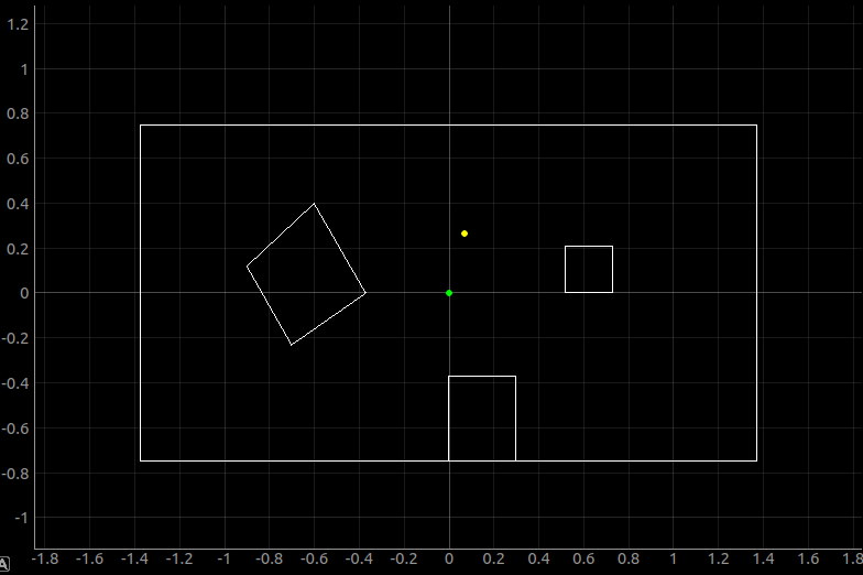
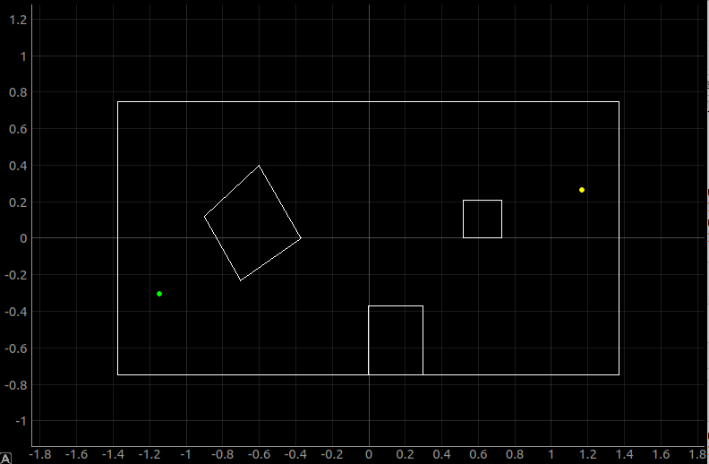
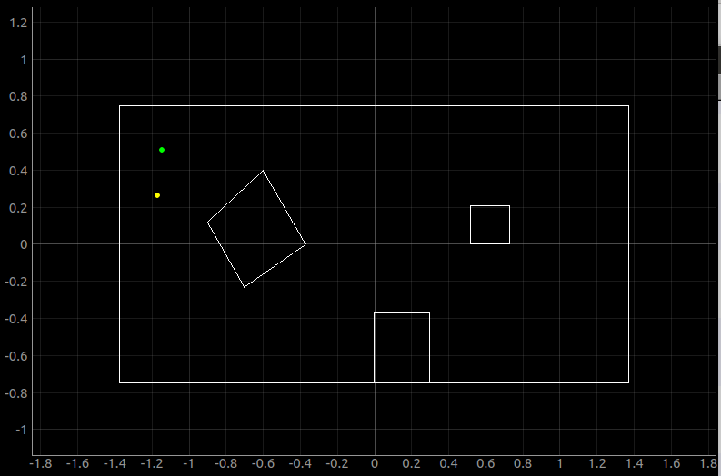
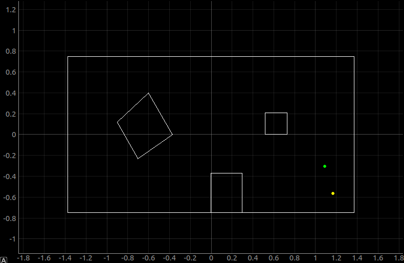
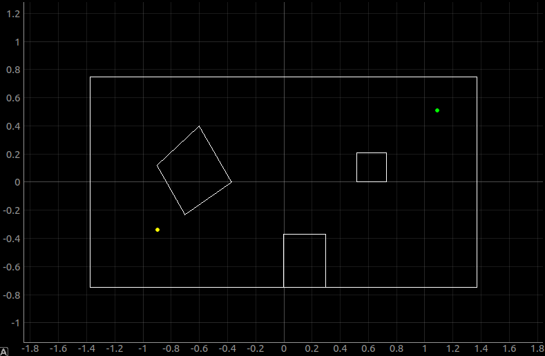
Figure 10: The five tests of the uniform experiment.
I also made a table in Figure 11 that shows the ground truth and the belief point in the update step. Therefore, I could conclude that if the environment was symmetry or too empty, having only the update step in the estimation would be not enough. The prediction step would consider the previous state and the current state to narrow the possible locations and improve the accuracy of the update step. Hence, I will do the second experiment to show the importance of the prediction step of the Bayes filter.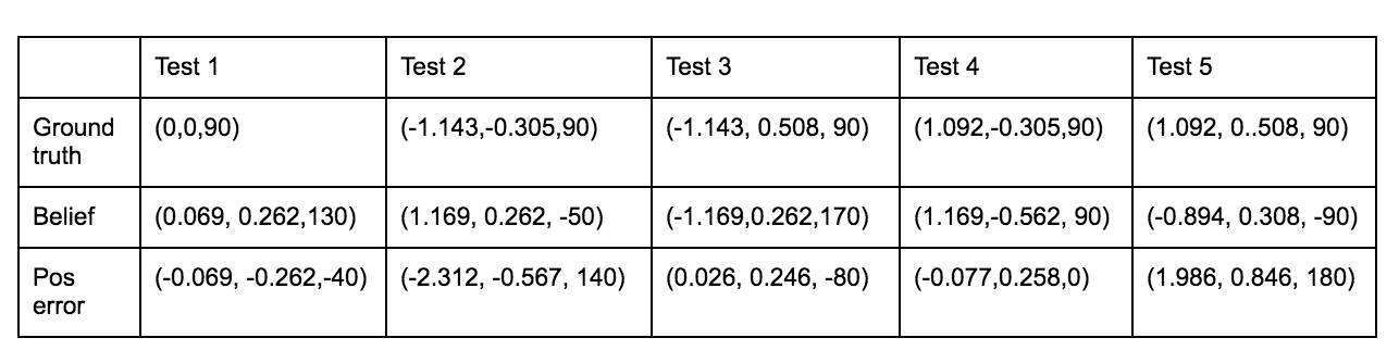
Figure 11: The update status of five tests.
In the beginning of the second experiment, I did three tests on the left side of the environment which contained four target points in order to see the repeatability and robustness of the program. The results show in Figure 12. I noticed that the deviation was huge because the odometry was quite noisy and the default odometry sigma value for the gaussian distribution was too small.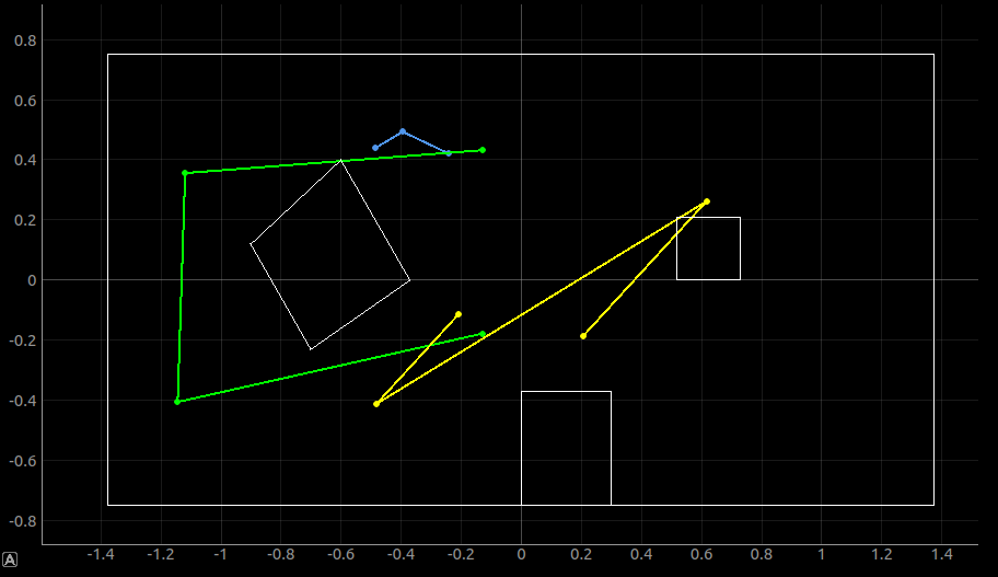
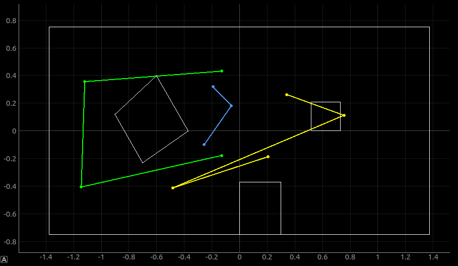
Figure 12: The two estimation trajectory with the default sigma.
Therefore, I tried to adjust the sigma value and observed the difference. I tried four different parameters which were trans_sigma = 0.1, trans_sigma = 1, trans_sigma = 1 with rotation_sigma = 60, and trans_sigma = 1 with rotation_sigma = 180. The results are displayed in Figure 13. I found that the small sigma will make the result become worse. The reason was that the sigma represented the standard deviation of the distribution, so the small sigma will allow only a small difference with the true value. Since the odometry was noisy, I decided to increase the sigma value for both transition and rotation to improve the tolerance of the Bayes filter. When I changed the trans_sigma = 1 with rotation_sigma = 180, it gave me the best result, so I used this parameter in my following tests.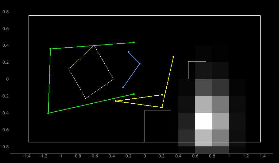

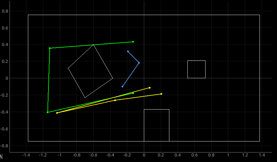
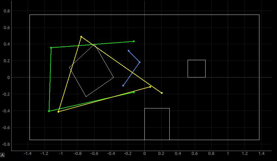
Figure 13: Different parameters of the sigma value. Top: trans_sigma = 0.1 (left), trans_sigma = 1 (right) Bottom: trans_sigma = 1 with rotation_sigma = 60 (left), and trans_sigma = 1 with rotation_sigma = 180 (right).
Once I set the parameter, I ran the three half-side tests again and the result was much better than the previous one. Although I changed the parameter, the results were still different from the true pose. Therefore, I adjusted the PID controlled rotational scan behavior to make the scan much slower and the radius of the rotation be smaller. It took me lots of time to adjust the motor’s speed because the motion was pretty noisy and was dependent on the battery charge.
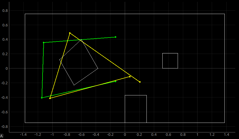
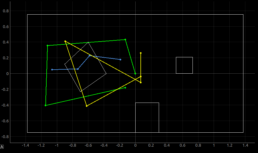
Figure 14: The estimation trajectory with the new parameter.
After I adjusted the robot motion, I made the robot go through the entire eight points and collected the data to run with the Bayes filter. Video 2 shows the process of the Bayes filter estimation and Figure 15 shows the result of the estimation trajectory with the true position. The execution time of the process was around 13.5 seconds.Video 2: The demonstration of the Bayes filter process.
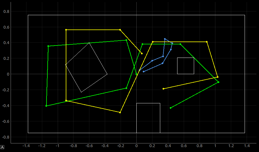
Figure 15: The Bayes filter result from the entire trajectory.
Note: The log of the Bayes filter, please click here .My inference of the result
I was satisfied that the estimation trajectory looked well. Although there was still a deviation between the true trajectory and the estimation trajectory, the result gave the robot estimated localization. I believed that the major influence of the result was the data fed to the classifier. The odometry information was too noisy and the measurements were not evenly measured. I considered that there were three ways to improve the result. First, using a specific speed for the robot to calculate more accurate odometry data. Since the yaw value was unstable, the entire odometry information would be inaccurate. Figure 16 shows the odometry function that I used in my program, which could see that the calculation was based on the yaw value. Second, tuning the PID controller parameter was important. The 18 measurements should be equally spaced, so it may be helpful to build a feedback function to ensure the robot to have the measurements properly. Third, adjusting the classifier parameters was critical. Once the odometry data becomes more accurate, the sigma value should be adjusted. Also, the threshold value inside the prediction step should be adjusted as well in order to reach the equilibrium point between the execution speed and the estimation accuracy.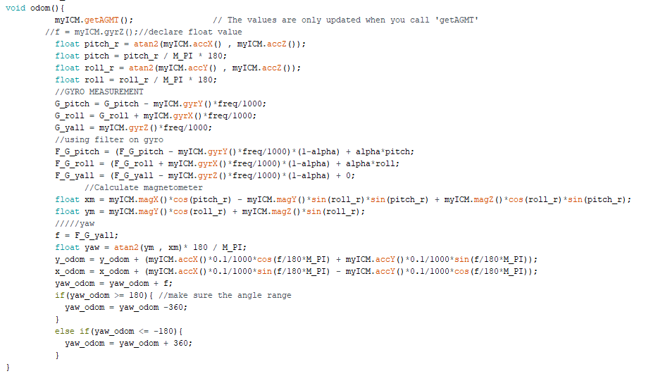
Figure 16: The odometry function in the robot.