Fast Robots: ECE 4960 Lab 3
In this week of the lab, we are going to understand the characteristics of the RC car. We will do simple measurements and set up several experiments to understand the capabilities of the car. Besides, we want to see the performance of how humans can control the car accurately. The overview image of the RC car we used in the lab shows in Figure 1.
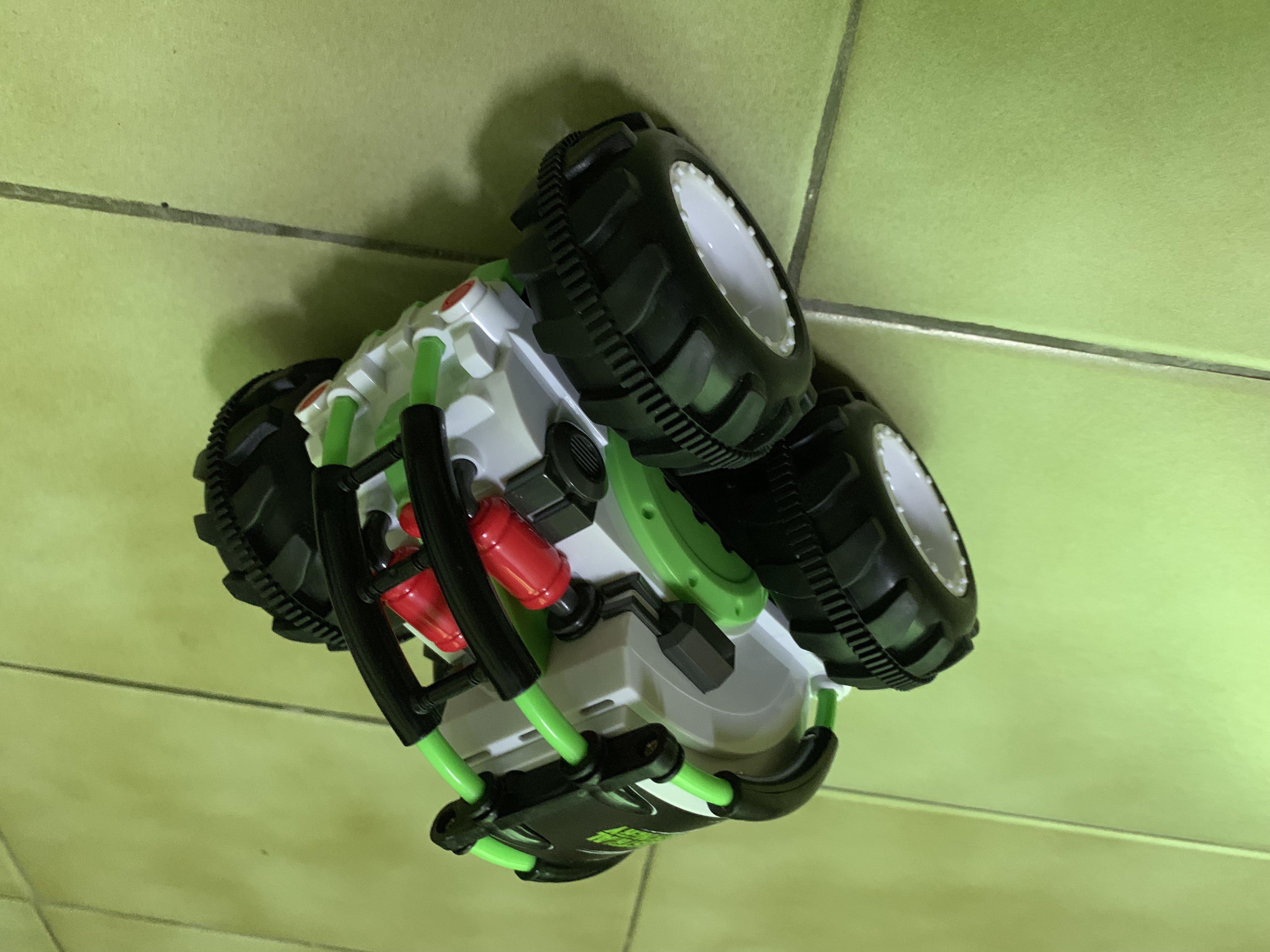
Figure 1: The overview of the RC car.
We will remove the upper case of the car to do the test because we will attach several chips on the car platform in the later labs. The car outlook is shown in Figure 2.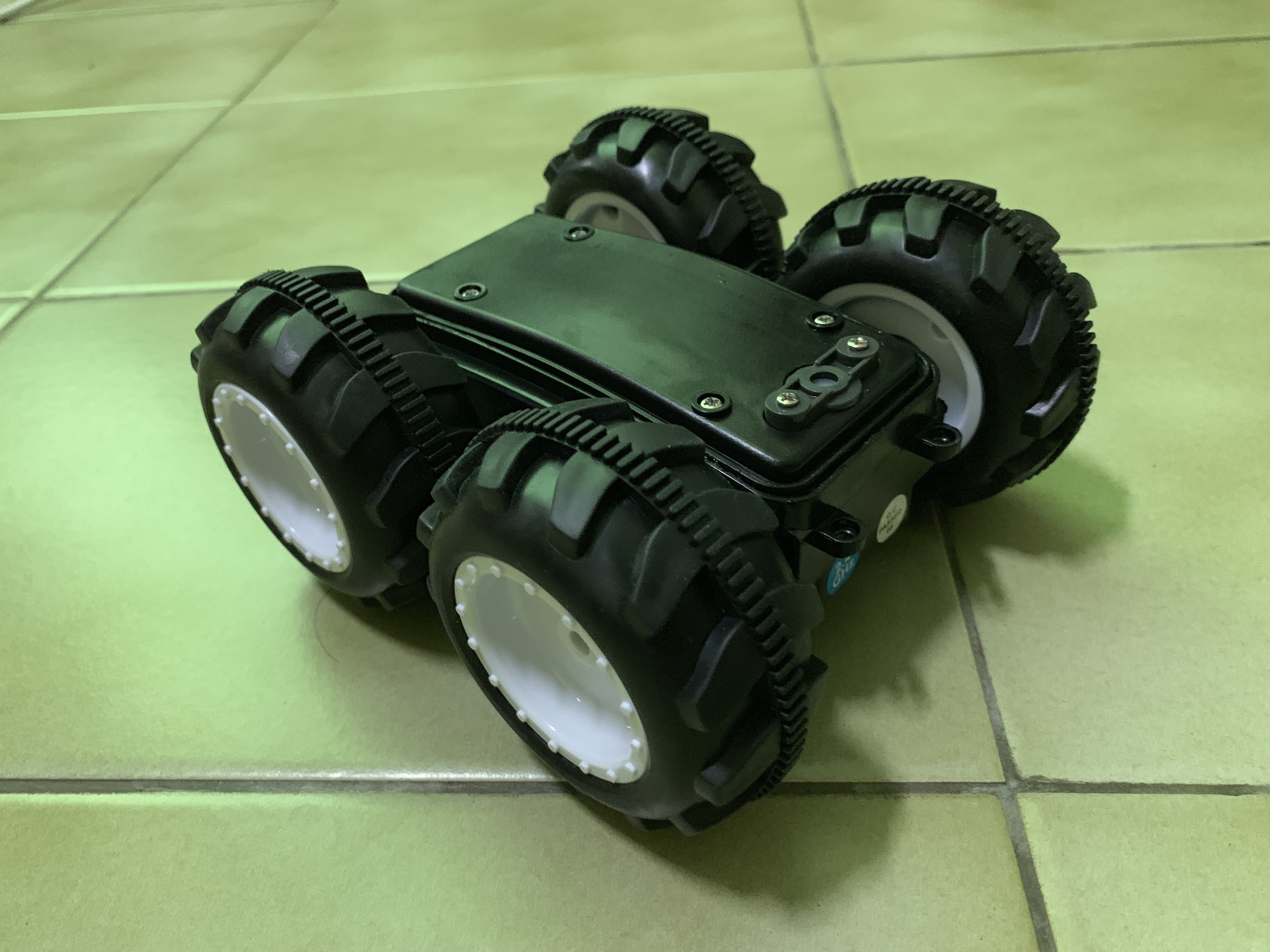
Figure 2: The RC car without the case.
Simple measurements
In this section, we will do several simple measurements to understand the characteristics of the car.Q: What are the dimensions of the car?
From Figure 3, the dimensions of the car is 15.2 cm x 13.3 cm x 7.5 cm (length x width x height).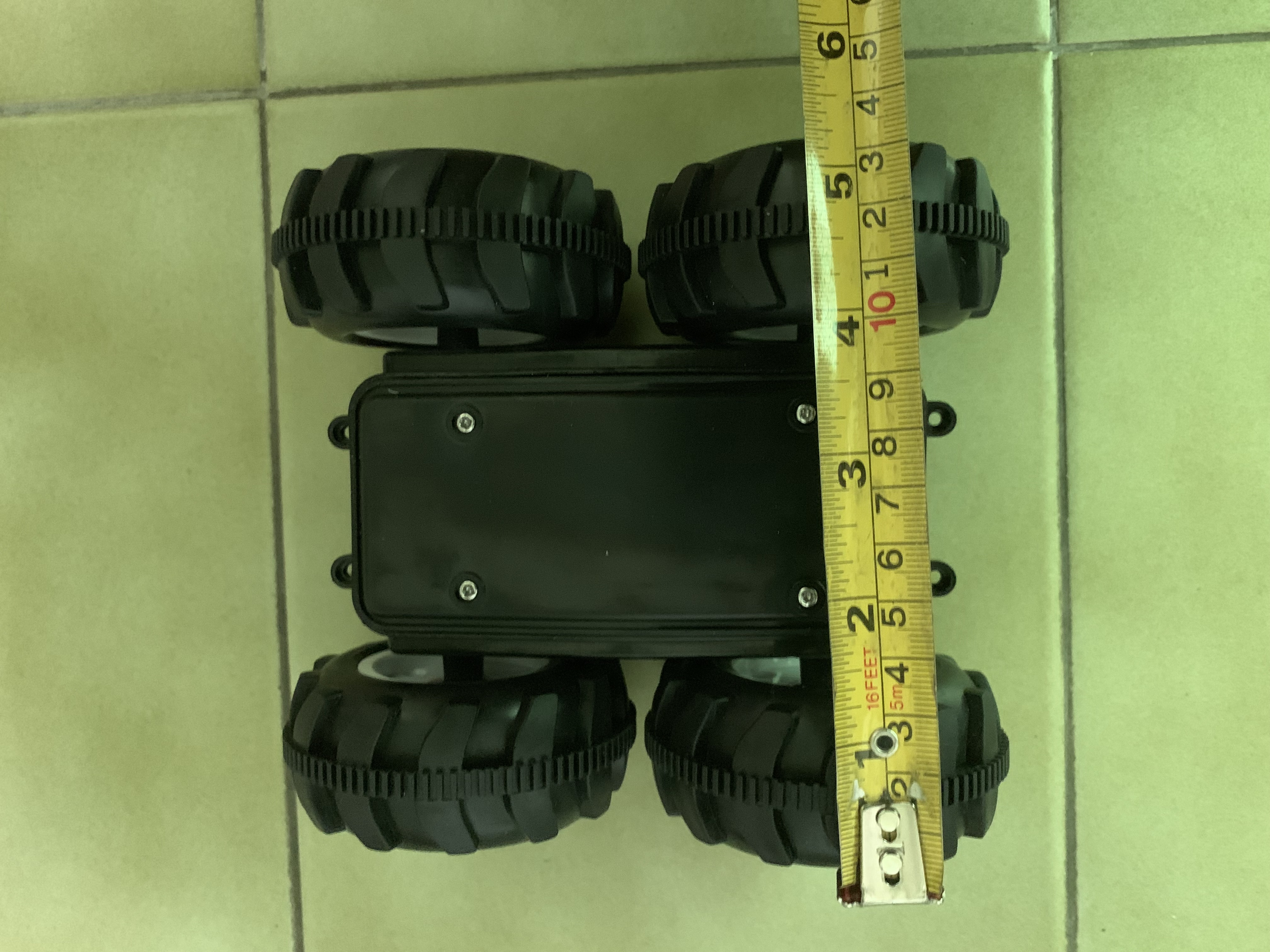
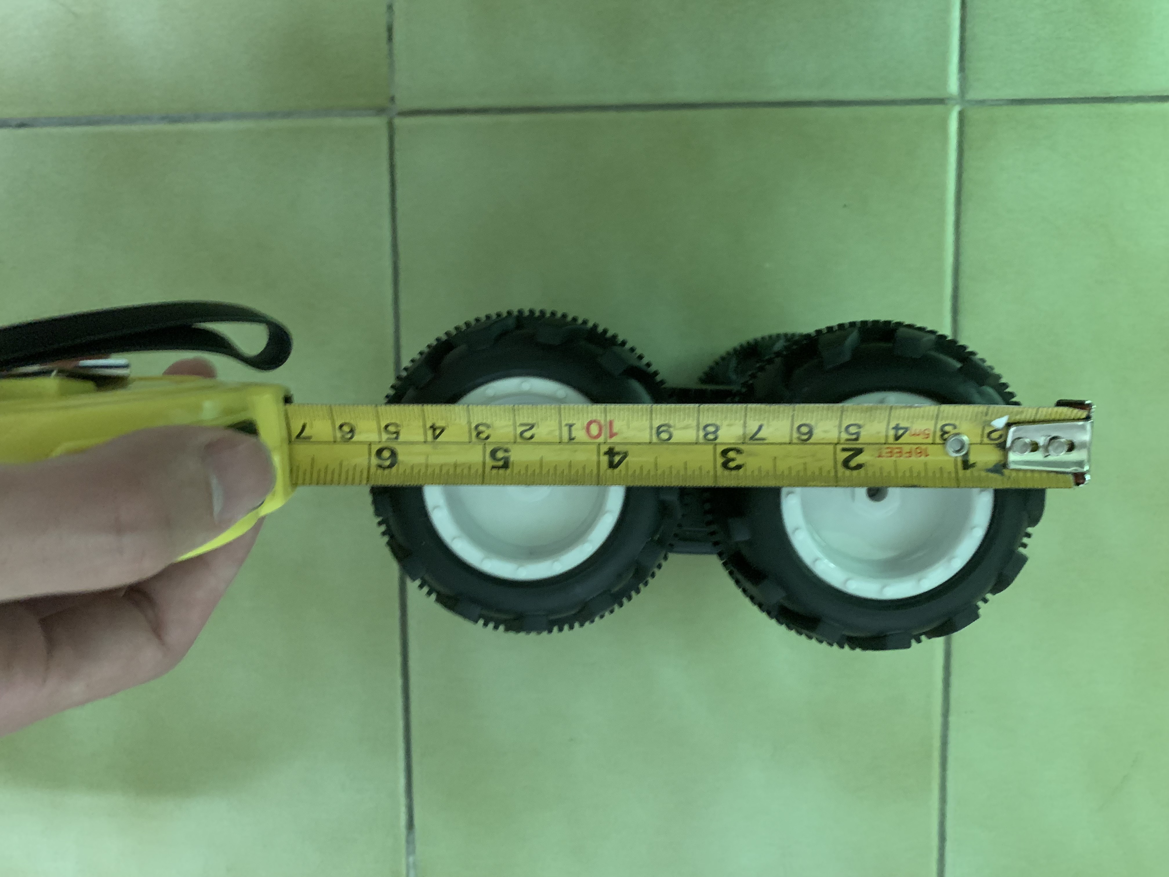
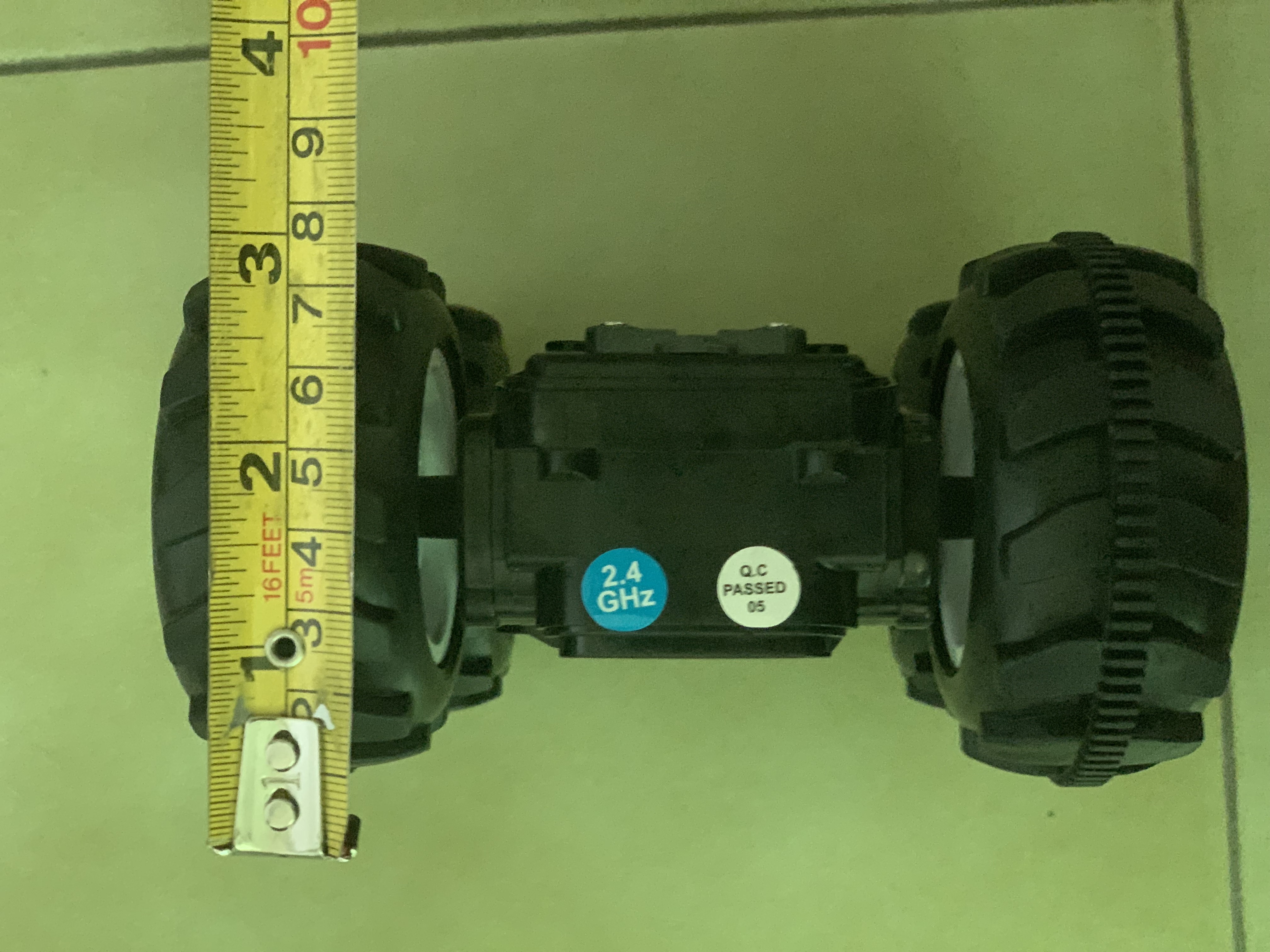
Figure 3: The length of the car (left), the width of the car (center), the height of the car (left).
Q: What is the weight?
From Figure 4, the car’s weight with a battery is 431.5 grams and the car’s weight without a battery is 367.5 grams.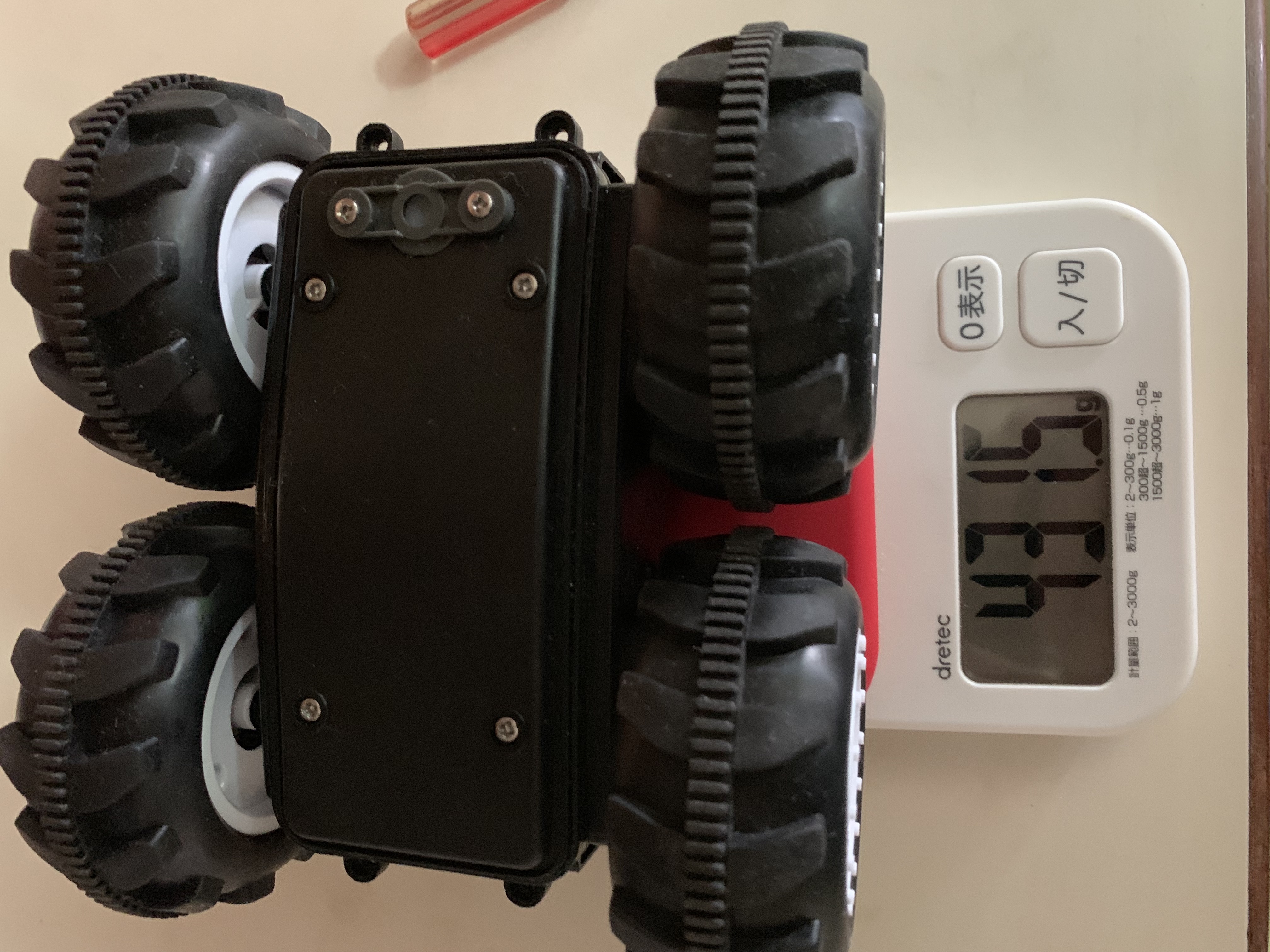
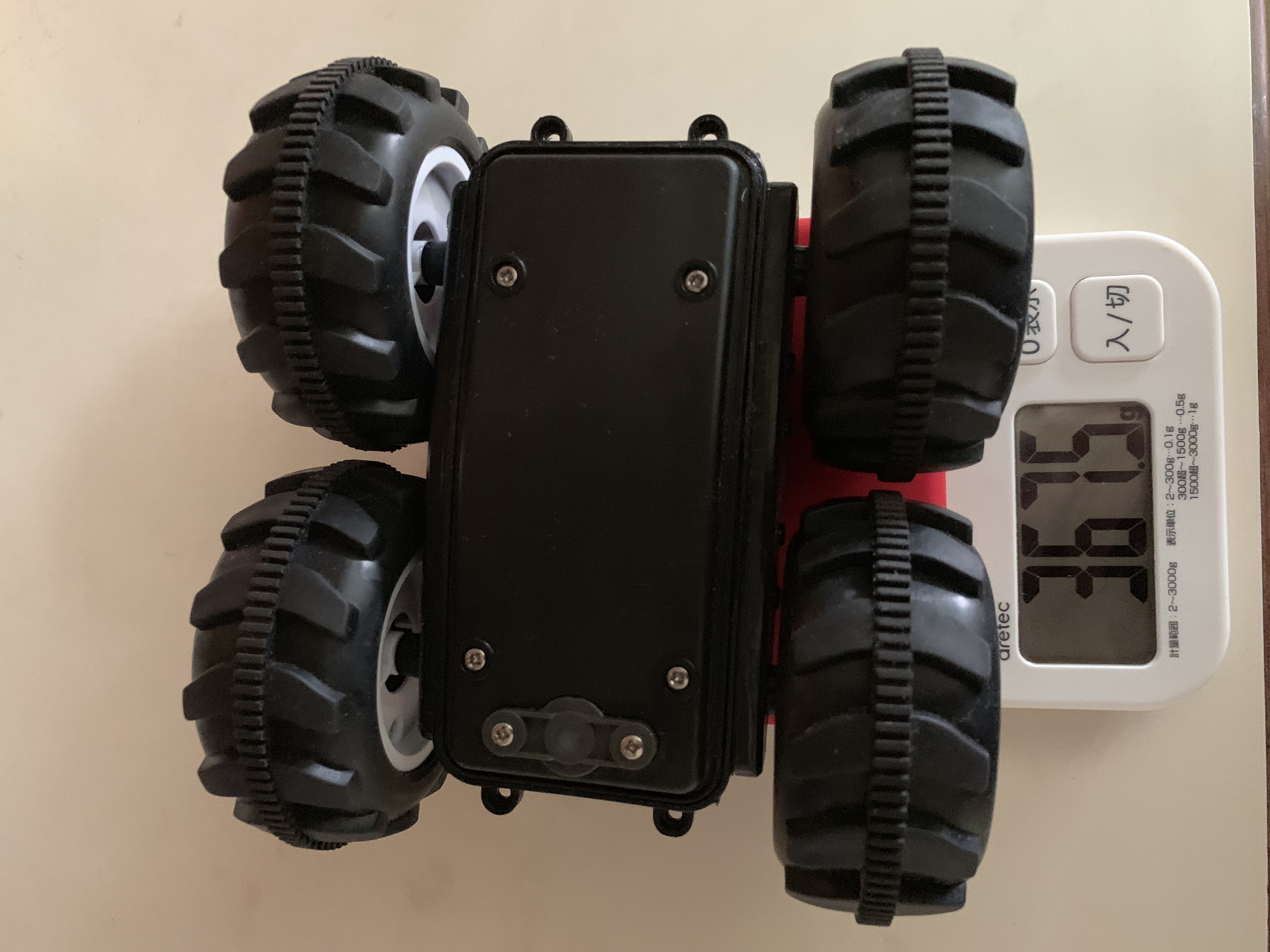
Figure 4: The weight of the car without a battery (right), The weight of the car with a battery (left).
Q: How long does it take to charge?
The power of the battery charger is 250 mA, and the battery we used is a 700 mAh Ni-Cd battery. Therefore, the theoretical time to charge the battery with 20% Efficiency Loss is 3.36 hours. The actual time we charged the battery is almost 4 hours.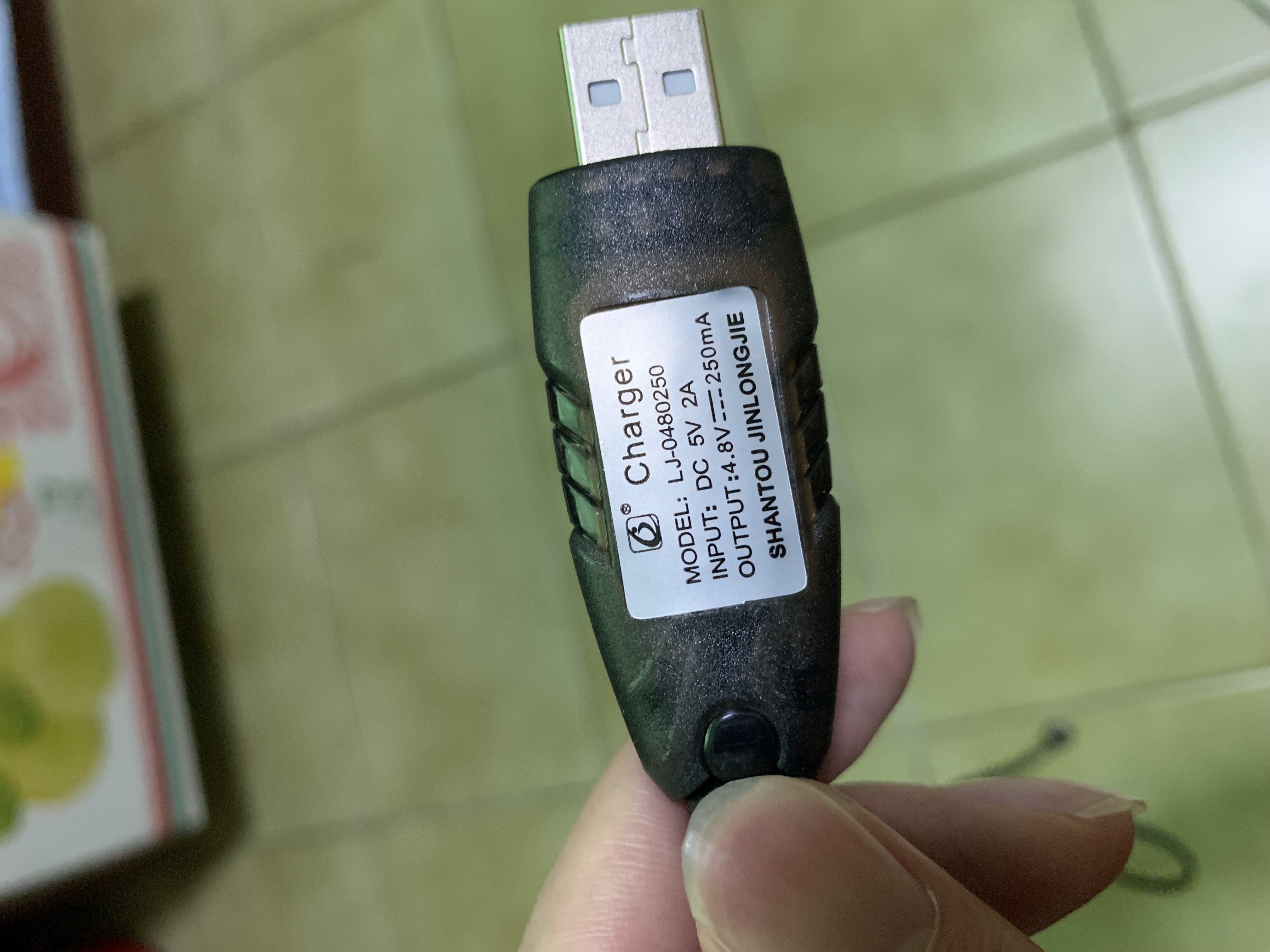
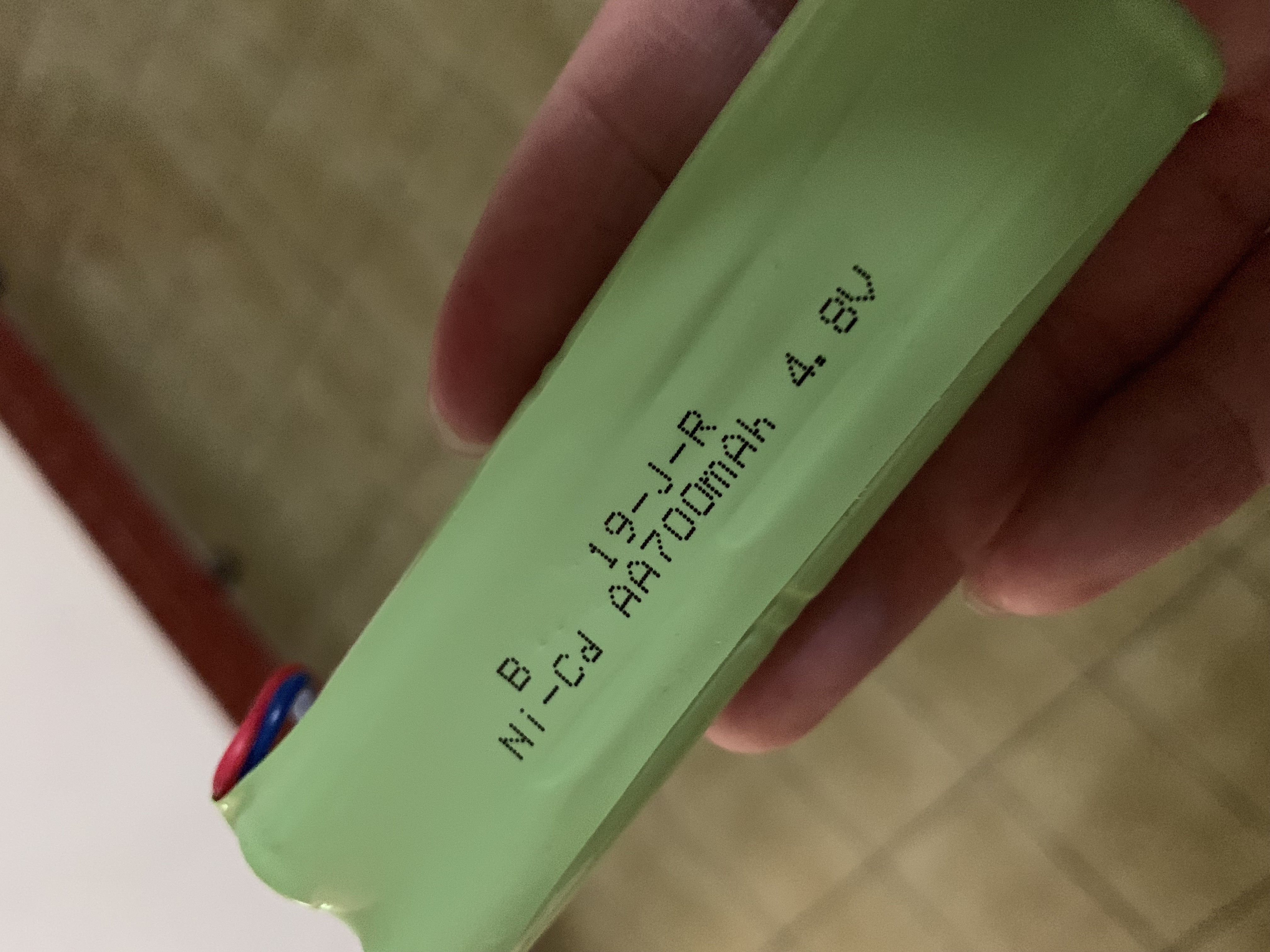
Figure 5: The charger (right), The battery (left).
Q: What is the battery lifetime?
The battery life for the car to run at full speed is about 18 mins, so we could determine the device consumption is around 2500 mA.Robot performance experiments
In this section, we will set up several experiments to observe the car behavior and record the experimental data for the following labs. In order to test the speed performance of the car, we set up the testing environment which is shown in Video 1. The yellow ball is the starting point, and each purple ball distance is one meter long. The red ball is a middle point, which indicates the five meters distance from the starting points.Video 1: Testing environment tour.
Q: What is the range of speed?
In order to calculate the speed range, we record each time when the car passed one meter long, so we can understand the speed for every one meter. We could see the speed plot and the distance plot for the five testing-sets in Figures 6. Besides, we got the average speed by dividing the total distance with the total time. The range of the speed we got is from 0.6757 m/s to 3.4483 m/s and the average speed is 2.26 m/s. It is quite slower than the value (4.1667 m/s) that shows on the company’s website, but we believed that it was the experimental error and our data is still reliable in the real world.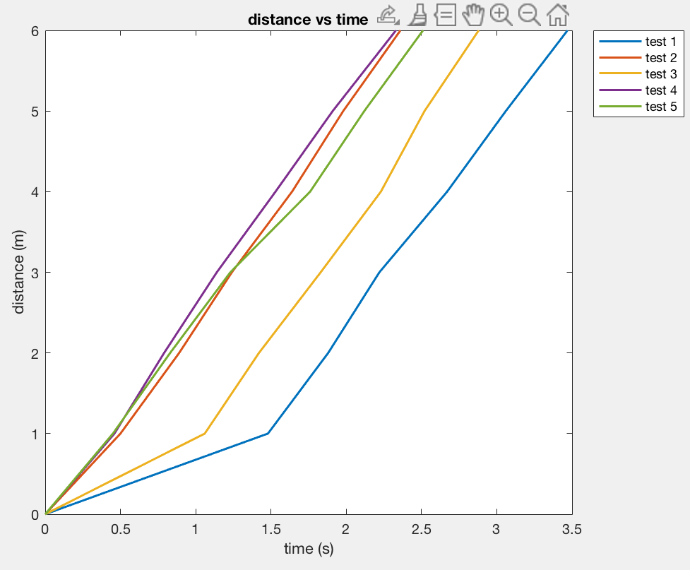

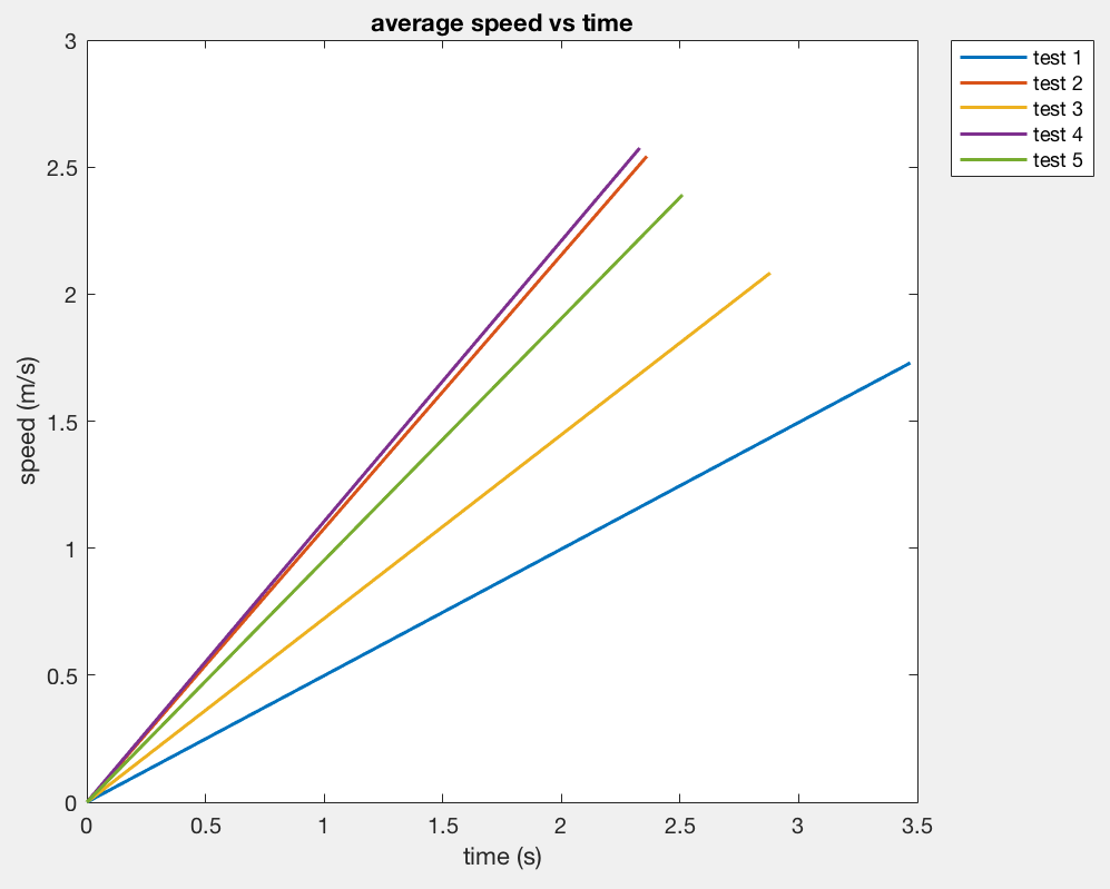
Figure 6: The distance vs time graph (left), the speed vs time graph (center), the average speed vs time graph (left).
Moreover, we realized that there is a speed-on button that can be pressed, so we repeated the same process, and we got four effective data. The plots are shown in Figure 7. The range of the speed we got is from 2.083 m/s to 3.33 m/s and the average speed is 2.519 m/s, which is faster than the previous test, so the speed button does work properly.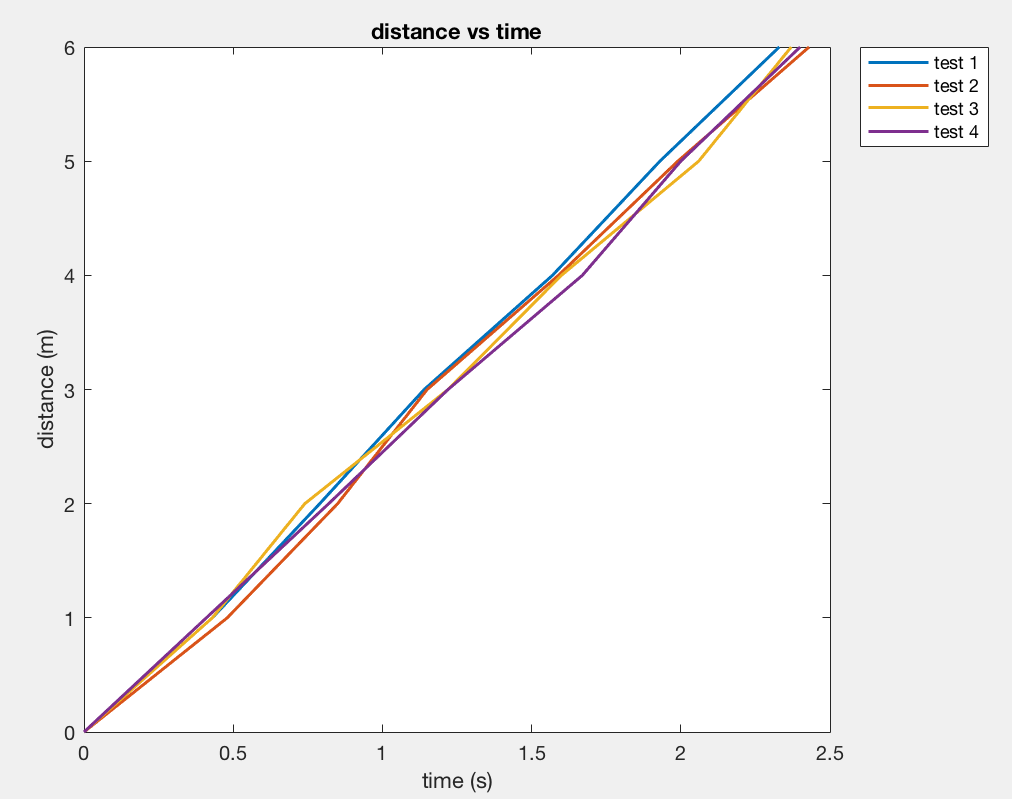
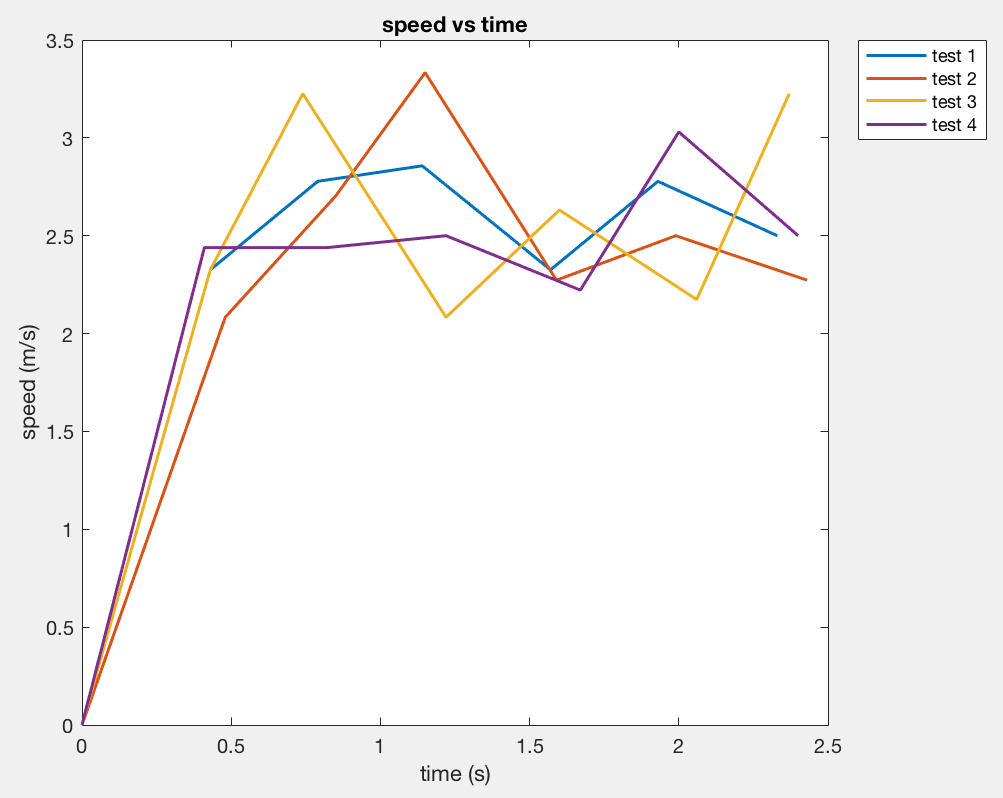
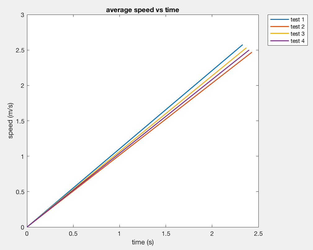
Figure 7: The distance vs time graph (left), the speed vs time graph (center), the average speed vs time graph (left).
Q: What is the range of acceleration?
Next, we divided one meter with each time to get the acceleration (we assume the acceleration is constant) for every meter. We could see the acceleration table in Figure 8 (right), and the range is from 0.4565 m/s^2 to 11.89 m/s^2. If we took the average acceleration, the value is 0.87 m/s^2 of these four tests. The figure is shown in Figure 8 (left).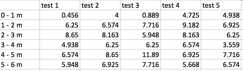
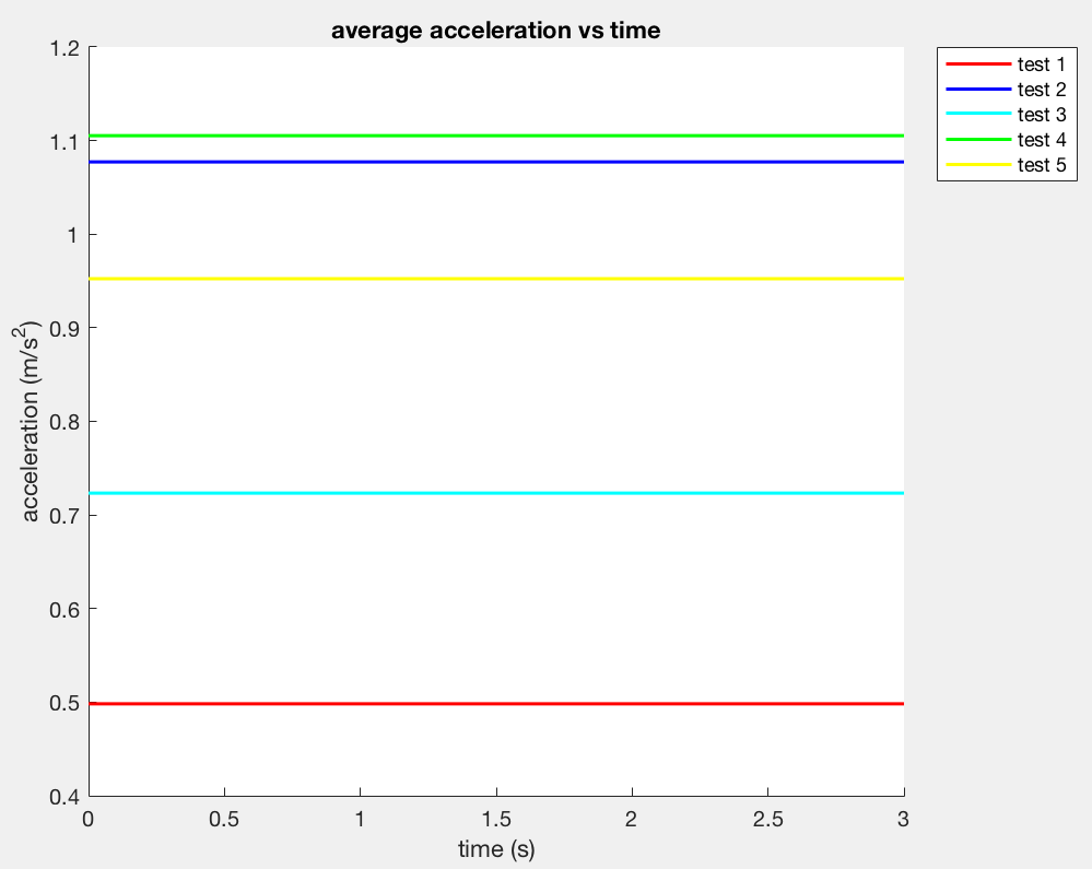
Figure 8: The table of the acceleration in every meter (right), The average acceleration for five tests (left).
We also tested the acceleration with the speed button and the acceleration table in every meter is shown in Figure 9 (right) and the average acceleration plot is in 9 (left). The range of the acceleration is from 4.34 m/s^2 to 11.11 m/s^2 and the average acceleration is 1.0578 m/s^2.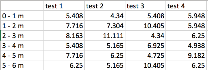
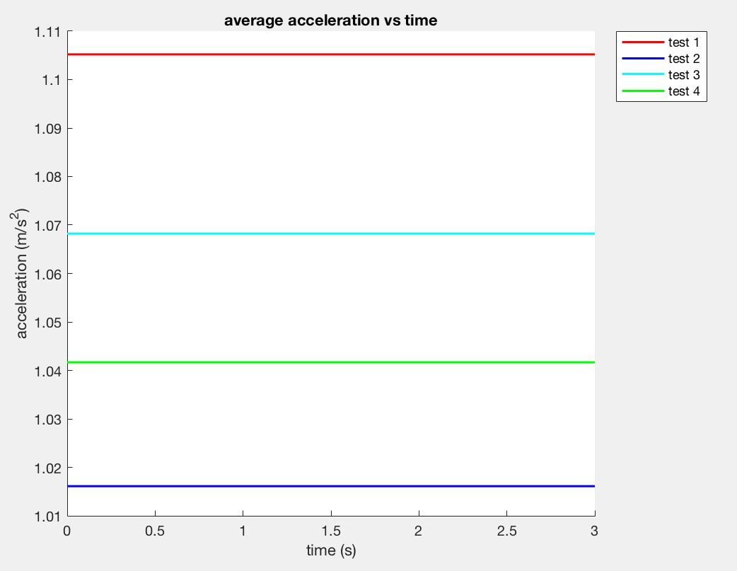
Figure 9: The table of the acceleration in every meter with the speed button (right), The average acceleration with the speed button (left).
Q: What is the braking distance?
In order to calculate the braking distance, we make the car run at full speed from five meters away and start to stop the car when the car passed the red ball. We will record the time from the start point to the red ball and the time from the red ball to the endpoint. The distance vs time plot is shown in Figure 10 (right) and the table in Figure 10 (left) shows the data. From the data, we could see the values of the braking distance are different, but the braking speed for the first three tests are pretty close, so we took these three values and calculated the braking force is 71.3 N.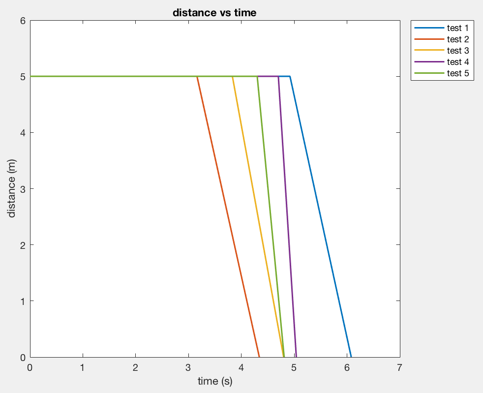
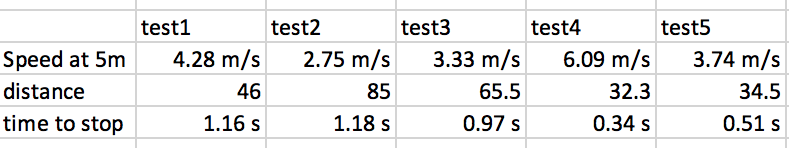
Figure 9: The distance vs time plot of the braking (right), The table of the braking data (left).
Q: What surfaces can it handle?
I have tested the car on the cloth sofa, indoor ceramics floor, plastic platform, and the asphalt road. The car can handle pretty well because its wheel has large friction to climb on the different surfaces.Video 2: Testing on the cloth sofa.
Video 3: Testing on the plastic platform.
Video 4: Testing on the asphalt road.
Q: What stunts can it do?
The car has two sides motors, so it can do a spin, 360 torments, and one sides standing, which shows in Video 5.Video 5: Stunts Capabilities.
Q: How reliably does the robot turn around its own axis?
From the Video 6, we can see the robot can turn rapidly with a slight offset of its own axis. We put some white powder on the car’s wheel and measure the distance of the offset. The average offset in 3 datasets is 2.3 cm.Video 6: Testing car turning axis.
Q: How well can you operate the car with manual control?
It is important to see the performance of the car with manual control. The first experiment is to start the car at a five meters distance and run at the full speed. The user will try to stop the car without a crash. We tested three times and the distance from the car to the wall is 10.3 m, 8.4 m, and 5.3 m, so the average distance is 7.33 m.Video 7: Obstacle test.
Next, we set up a meter-scale square with four balls in four corners separately. There are four effective data and the times are 9 sec, 6 sec, 8 sec, and 9 sec, so the average time is 8 sec. It is hard for humans to hit four corners accurately at a high speed. The best testing set is shown in the following video.Video 8: Four corners test.
Then, we want to reproduce the tricks that we found the video on the tricks website. In Videos 9 and 10, we reproduced the lazy headslide and spindive 540. We have to prepare a jumping platform and run with a full speed to have the lazy headslide. On the other hand, the spindive is pretty similar to the lazy headslide, but we need to immediately change the wheel directions before the car jumps out of the platform.Video 9: Lazy headslide.
Video 10: Spindive 540.
Last, we tried to see the balance of the robot. We made the car go forward at full speed and suddenly go backward, which is shown in Video 11. We can see the car can stand with one set of wheels at a period of time, but the time is vary depending on the surface.Video 11: One wheel test.
Simulator tests
After we played around with the RC car, we started to set up the virtual robot in the simulator, so we could test the robot’s performance in order to prevent errors before setting up the RC car in the real world. We will need to install the “ros-melodic-rosmon” library in our VM, but there is an error while installing, which is shown in Figure 10.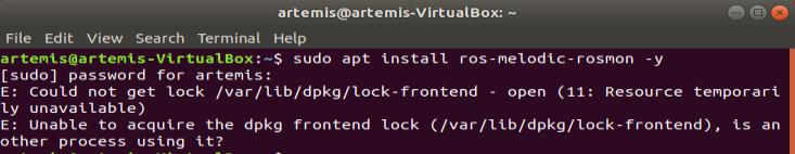
Figure 10: The error message for installing the library in the terminal.
In order to fix the issue, we have to set up the “Software & Updates” menu in the right order, which shows in Figure 11. Once we updated the setting, the library could be installed properly.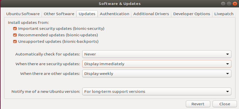
Figure 11: The setting of the updates.
Next, we downloaded the simulator program from the course website and compiled it in the terminal that shows in Figure 12.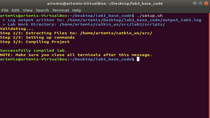
Figure 12: The compile process of the simulator.
Once the simulator has fully set up, we could run the lab3-manager command in the terminal to start the simulator. The simulator environment is displayed in Figures 13.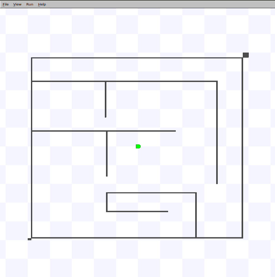
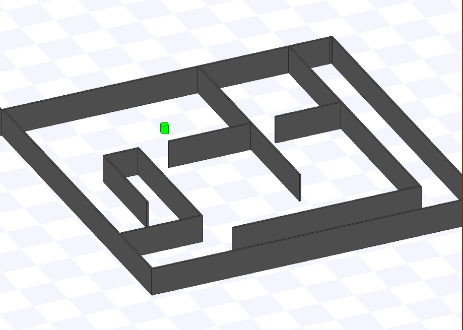
Figure 13: The 2D image of the map (right), the 3D image of the map.
Then, we could run the command “robot-keyboard-teleop” in the new terminal, so we could control the virtual robot with the keyboard. We played around with the various toggles of the simulator and tried to observe the control performance of the robot. We realized that the linear and angular speed can go to infinitely small, but the minimum value for us to observe is that 0.000106 m/s for the linear speed and 0.01278 m/s for the angular velocity. Besides, we tried to kidnap the robot while it is moving. We noticed that the robot can still move in the same direction once it was placed in the other location. However, if the robot bumps into an obstacle, the robot symbol will turn into an exclamation mark. The robot will stop until the user moves it to the free space of the map. The demonstration is shown in the following video.Video 12: Simulator demostration.