Fast Robots: ECE 4960 Lab 8
Objective
The purpose of this lab is to implement grid localization using the Bayes filter. I will take the TA’s feedback and update the precursor program that I wrote in lab 7. After verifying the Bayes filter program, I will operate the Bayes filter for the entire trajectory which may take around 5-10 minutes. I will record the time to see how efficient my code is. I will also point out the difference between the new code and the previous code by comparing the estimation results.Implementation
According to the feedback I received from the TA, Vivek, my compute control and the odom_motion_model function looked good, so I did not modify the functions, which can see in Figures 1 and 2.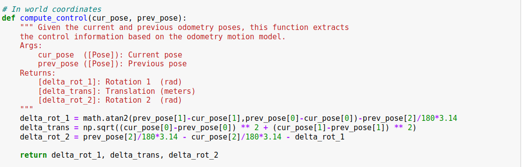
Figure 1: The code of the compute control program.
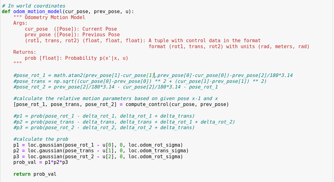
Figure 2: The code of the odometry motion model program.
In the previous prediction function, I only considered the estimation position that I got from the update step, and calculated the belief bar for the entire grids. However, this process was not correct although the result looked well. The correct prediction step should iterate over all previous and current states. For example, the current cell (0,0,0) should compare with the entire grids and calculate the probability of each cell, so it will need to take 7200 loops to finish the calculation for one iteration and 51 million loops for all the grid. It will be a lot of computation for one prediction step. In order to make the estimation process to run more efficiently, I will set a threshold value to filter the states that have small probabilities because those states don’t contribute a lot to the belief. However, it is important to normalize every time I compared a previous state with the entire current state to ensure that the entire grid has a sum to 1. If the normalization was implemented wrong, the result will look like the trajectory in Figure 3. So, the completed prediction function shows in Figure 4.
Figure 3: The wrong trajectory with the wrong normalization placed.
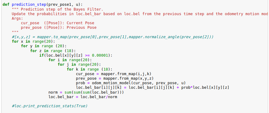
Figure 4: The code of the prediction step.
Next, I removed the normalization in the sensor_model function. The normalization should happen after incorporating the measurement likelihood into the belief, which should be in the update step function. The function shows in Figure 5.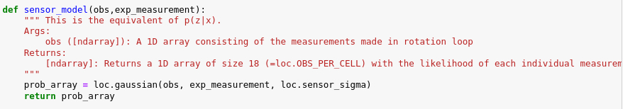
Figure 5: The code of the sensor model.
Last, I did not change the update function. I knew that the update function would call the sensor-model function to get 18 probabilities of 18 different individual measurements. Each individual measurements are independent given the robot state, so the total probability should be a multiplication of the probabilities of each measurement. I normalized the belief after the computation to prevent arithmetic underflow. I tried to move the normalization into the loop and I found that if I normalized the belief every time I calculated a cell, it will be inaccurate because the normalization may make the signal small number becomes larger without considering the entire girds distribution. For example, if I got the value 0.001 and normalized it, the probability of the cell will be one. If I did the normalization with a grid that had the value 1, 0.01, 0.05, and 0.001, then the cell that has the value 0.001 will still be small and not influence the estimation. So, I normalized only one time after the updated step was finished. The completed updated function shows in Figure 6.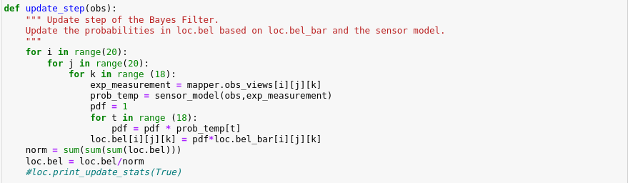
Figure 6: The code of the update step.
Result & discussion
After I finished all the functions, I did the same tests that I did in the last lab. I tried the linear motion of the robot and plotted the estimation to compare the result with the lab 7 plots, which shows in Figure 7. I noticed that the correct Bayes filter will quickly converge and have less offset to the truth pose, but the wrong filter will have large fluctuations. The reason was that the previous filter only considered a single position in the prediction step, so the correct estimation will be based on the update step. Once the estimation was really close to the true position, the expected measurement and the sensor measurement would be very similar, which leads the estimation to become reasonable. However, if the environment was symmetry or theP(z | x) was too similar, the estimation will be wrong.
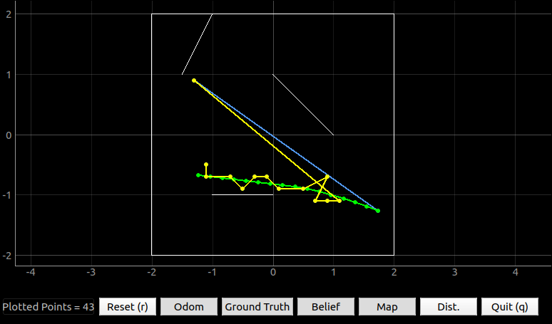
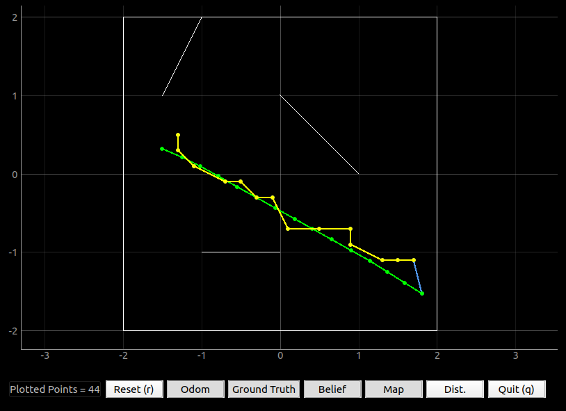
Figure 7: The comparison between the wrong filter (left) and the correct Bayes filter (right).
Next, I tested the threshold value and observed the factor effects. I tried the threshold value for 0.01, 0.00001, and 0.00000001. The result shows in Figure 8. I realized that the threshold value cannot be too larger. If the threshold value is too large, then the estimation will be inaccurate and the trajectory will be a sawtooth shape because the algorithm considers fewer possible locations of the grid in the prediction step. On the other hand, if the threshold value is too small, the computation will take too long for one iteration, so it is not realistic.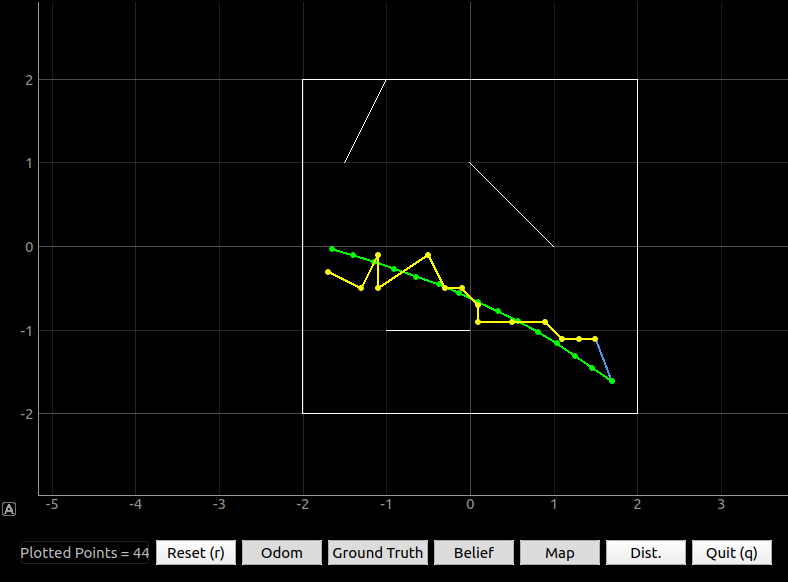
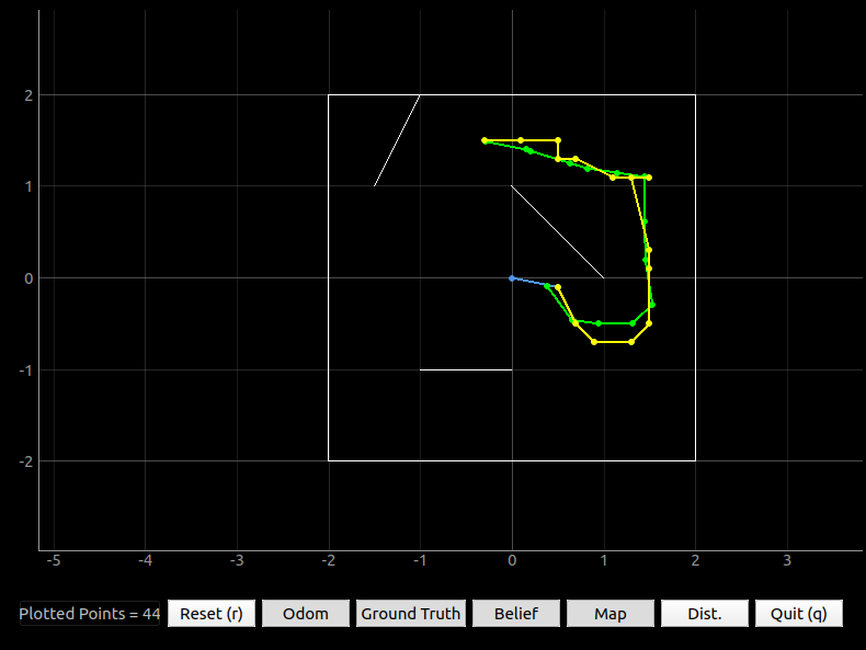
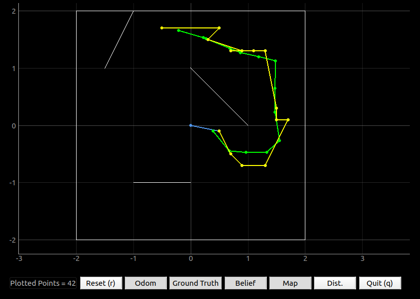
Figure 8. The comparison of different threshold values with linear and nonlinear motion. Top: Linear motion with threshold 0.01 (right) and 0.0001 (left); Bottom: Non-linear motion with threshold 0.01 (right) and 0.0001 (left).
Last, I ran the entire given trajectory three times and analyzed the repeatability of the estimation. I also record the elapsed time of the computation. The completed control function is shown in Figure 9 and the results show in Figure 10. I found that the Bayes filter worked properly and each estimation was closed to the truth pose. Besides, the elapsed time of each test was 433.592, 432.932, and 434.713 seconds. The average computation time was 433.746 seconds. If I want to reduce the computation time, I may need to sacrifice the accuracy of the estimation, so I decided to keep the current status for my Bayes filter. Besides, Video 1 and Video 2 shows the demonstration of the Bayes estimation with linear and nonlinear motion. I observed that the prediction belief would be updated when the updated step was completed, so I believed that my program worked properly and I am excited to implement the algorithm on my robot.
Figure 9: The main function of the Bayes filter.
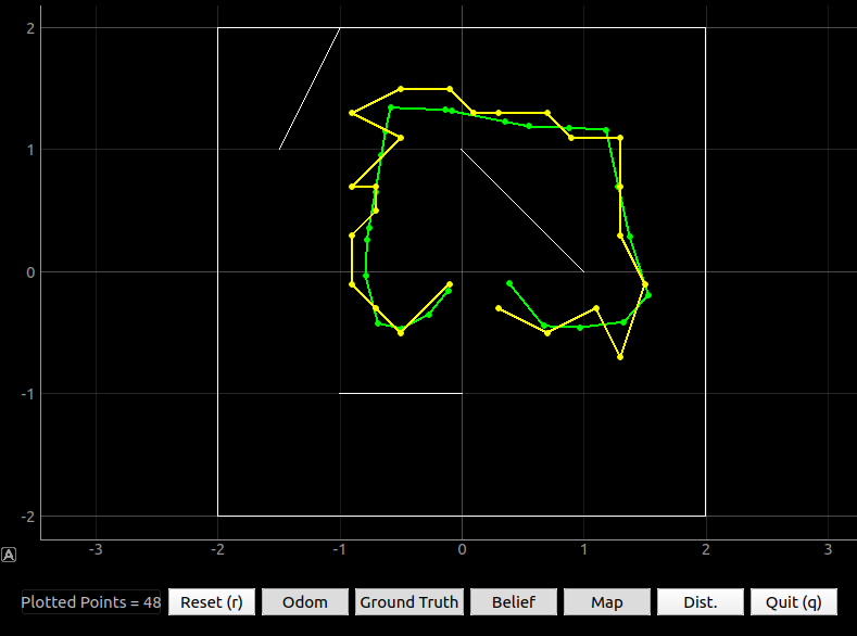
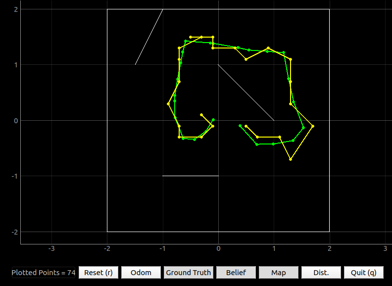
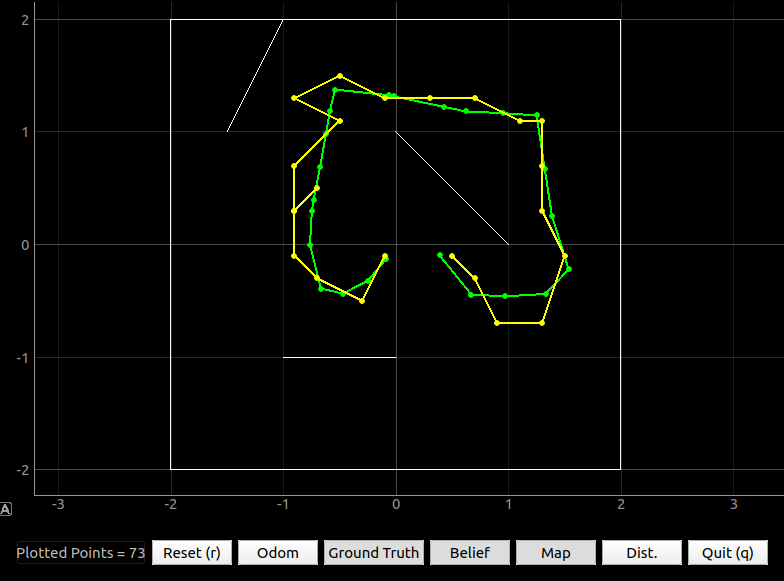
Figure 10: The three results of the completed estimation.
Video 1: The demonstration of the linear motion estimation.
Video 2: The demonstration of the non-linear motion estimation.
Note: Figure 11 is the odometry trajectory plot of the video and click here to see the prediction/updated log.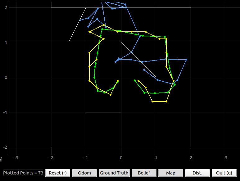
Figure 11: The odometry trajectory of the robot.