Fast Robots: ECE 4960 Lab 5

Objective

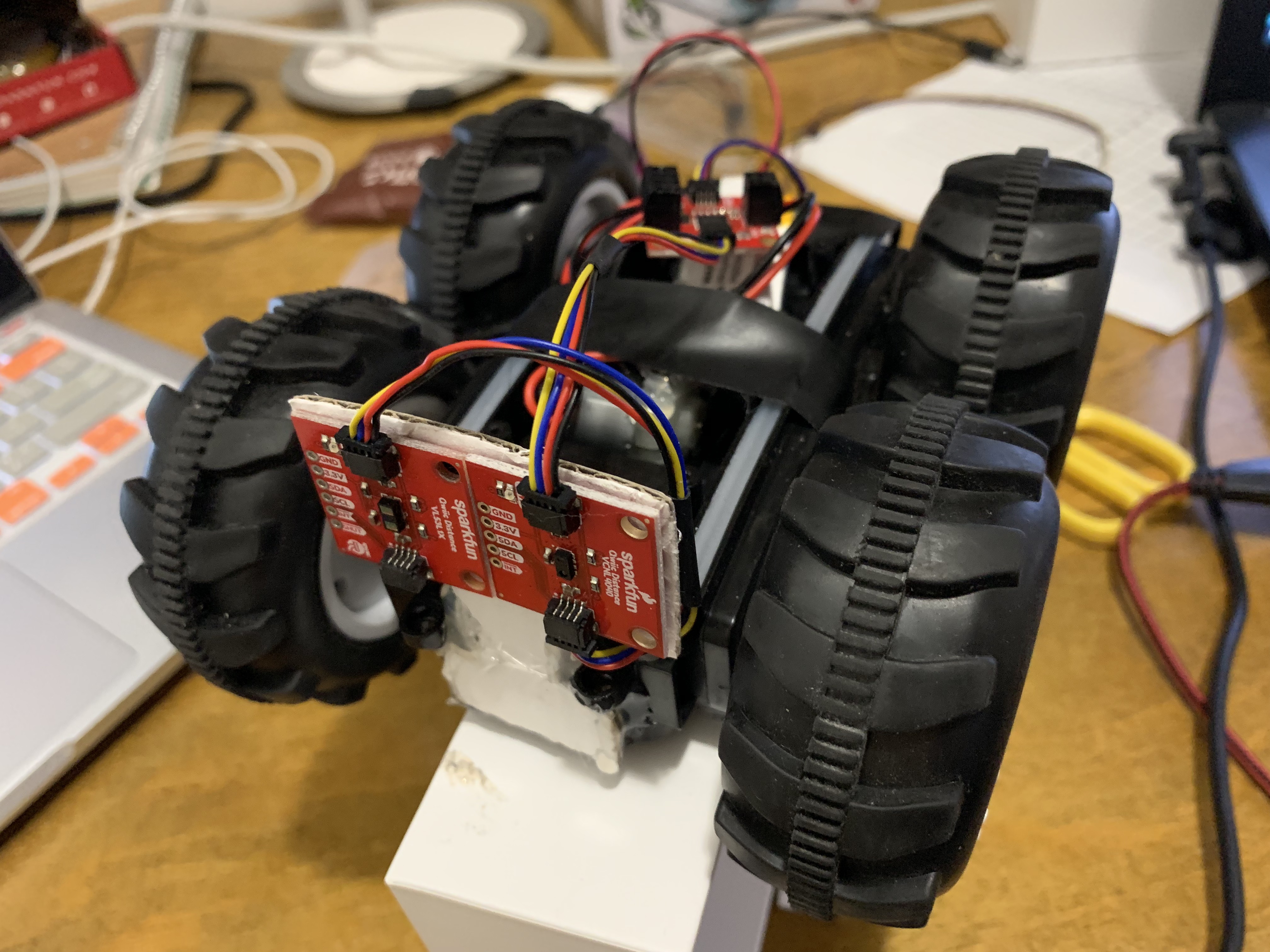
This week, we will implement the obstacle avoidance feature on our robot. We will need to test two sensors, which are proximity sensor and time-of-flight sensor, to understand the accuracy the respond time of the sensor. Once we learn how to use the sensor, we could modify the program and make the robot move fast as possible without crashing into obstacles. We will show our results in the real time and the simulator in two sections.

Proximity Sensor

The first sensor that we used is the SparkFun proximity sensor VCNL4040. We will use it to detect objects that is up to 20cm away. This sensor is a simple IR presence and ambient light sensor. We will connect the sensor with the Artemis board using a QWIIC connector. We could run the “wire example” from the library to check the I2C address. The slave address of the sensor is “0x60”, which is the same from the datasheet. To test the sensor performance, we tested three different color objects from the 20cm away from the sensor. The colors of the objects are black, purple, and white. In the Figure 1, we could see the color of the object will affect the sensitivity of the sensor. If the object is more colorful, it is more possible to be recgonized.

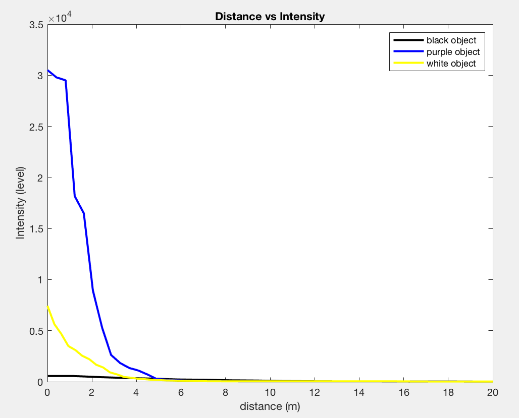
Figure 1: The intensity of the sensor within distance.

Besides, we want to see the respond time of the sensor, so we ran the example program (Example2_IsSomethingThere) and record a video to analyze the time. We found that the detection had an average delay at 3.4432 seconds, which is too long for the obstacle detection, but we realized that the elapsed time of the proximity detection was 0.0579, so we believe that it was the algorithm that caused the delay. We will redesign an algorithm and discuss it in the experiment section.

Video 1: The respond behavior of the proximity sensor.

Time of Flight Sensor

The second sensor we used is the SparkFun VL53L1X. It is the next generation of ToF sensor module that has high accuracy at long ranges. We are able to use the sensor to he distance to an object from 40mm to 4m away with millimeter resolution. We will use a QWIIC connector to connect the sensor with the proximity sensor. We use the wire example program to check the I2C address, which is “0x29”. The address matches with the given datasheet. Before we start testing the sensor accuracy, we ran the calibration program to calibrate the sensor, which shows in the Figure2. We could see it has an offset 139 within a short distance from the sensor, so we applied the offset to the program for the further tests.

Figure 2: The calibration of ToF sensor.

Besides, we need to understand the characteristics of the sensor, so we played around with the examples from the library. We noticed that if we adjusted the intermeasurement period of the sensor, the measurement respond time will become slower. In order to avoid obstacles in the real-time, we decided to use the default time (100ms) in our program. Also, the signal rate of the sensor will be dependent on the object’s moving speed. If the object moved rapidly, the signal rate will be smaller and cause the failure of data wrapping. To prevent this scenario, we will use the proximity sensor to assist the ToF sensor in order to improve the trustworthiness of the reading. Next, we tested the elapsed time of the sensor in three different conditions, which are ranging with stop, ranging without stop, and ranging without interrupt. The result is shown in Figure 3. As we expected, the ranging time without interrupt is the shortest, so we will use the code in our obstacle program to get an immediate response.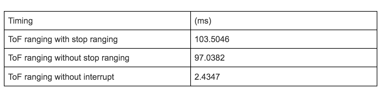

Figure 3: The table of the ranging time.

Last, we noticed that there are two modes (4m and 1.3m) for ranging. To understand the accuracy, we had tested the sensor with a stationary object every 25cm until 2m. After two meters, we tested 2.5 and 3m in order to compare the difference of two modes and the range ability. In Figure 4 (right), we could see that sensor has a high accuracy in both modes when the distance is less than two meters. The percentage of the difference between the measurement and the actual distance is 0.67% (long mode) and 2.51% (short mode). When the distance is larger than 2 meters, the long range mode still maintain a good accuracy but the short range mode has huge errors, which is shown in Figure 4 (left). Therefore, we will set the range in long mode in our design.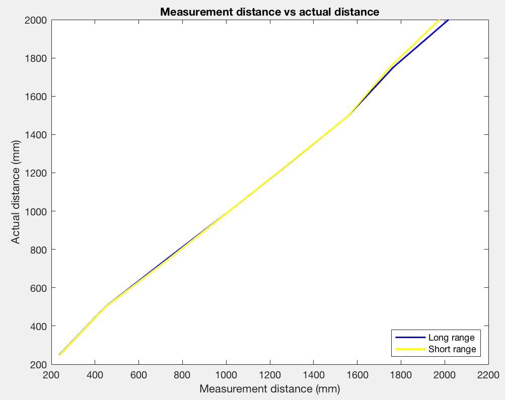

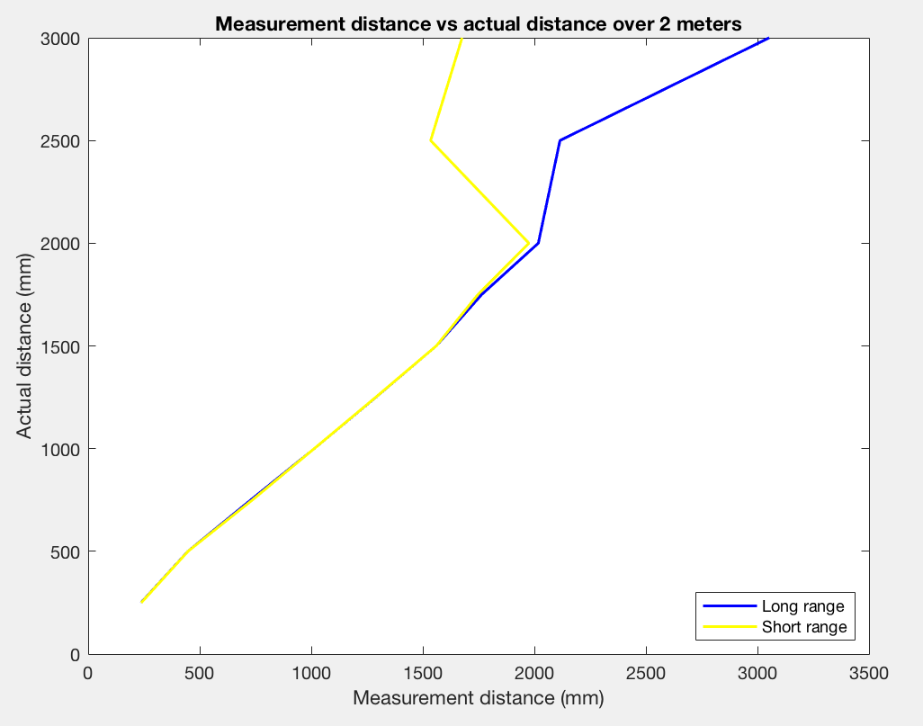
Figure 4: The measurement vs actual distance. Less than 2 meters (right). Larger than 2 meters (left).

Also, we put a stationary object one meter away from the sensor and measure the distance five times to observe the repeatability. We calculated the average distance for each tests in both mode and the results show in Figure 5. The number shows that the sensor has a high repeatability, so we could trust on the data reading.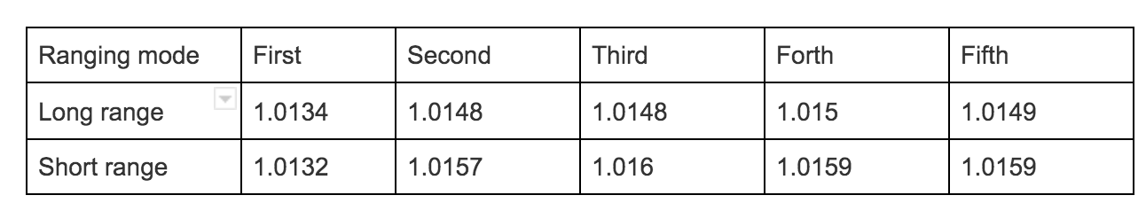

Figure 5: The repeatability of the sensor at 1 meter away.

Program Design

The purpose of this lab is to make the robot avoid hitting any obstacles. To achieve this goal, we make the robot stop moving while the program starts. The robot will detect whether there is obstacles that is less than 50 centimeters. Once the detection is completed, the robot will count the clock for five seconds before it starts to make sure that the road is clear in the front of the robot. The robot will start from its minimum speed that we calculated from Lab 4, which are 30 and 55. The robot will increase five of the speed every loop till the setting maximum (120 for our design) if the value that returns from the ToF sensor is larger than 1 meter. Once the ToF sensor detects the distance is less than 1 meter but is greater than 50 centimeters, the robot will start reduce its speed till its minimum rate. If the detect distance is less than 50 centimeters, the robot will backward for 0.3 seconds and turn a slight angle.While the robot is rotating, the ToF sensor will keep measuring the obstacle distance. If the distance is larger than 50 centimeters, the robot will start moving forward again. Additionally, the proximity sensor is used as a second protection while the robot is moving, but there is an obstacle that moves rapidly. The sensor will keep measuring the environment proximity and the program will store one proximity level of the previous state. It will compute the difference of the level between the current state and the previous state. If the level is 50% different, it will identify that there is a object, so the robot will stop and search for the new direction. The demonstration of the program is shown in Video 2. The Figure 6 shows the main loop of the program.

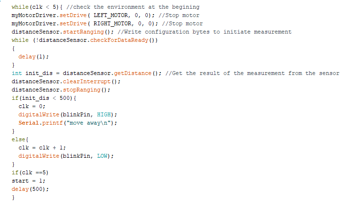
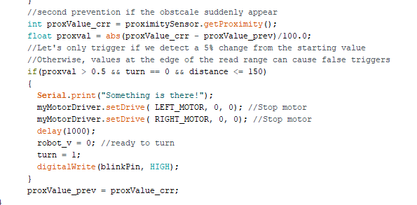
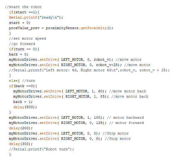
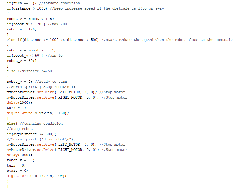
Figure 6: The obstacle avoidance program of the real-time test. Initial search (top left), Motor control(bottom left), Proximity measurement(top right) , ToF distance measurement (bottom right).

Video 2: Obstacles avoidance program demonstration.

Real-time testing

In Video 3, we could see our robot can successfully avoid the obstclae and it will find a suitable direction to continue moving. Also, it shows that the robot will increase speed if the obstacle is far away and reduce speed if the obstacle is getting closer. In Video 4, it shows that the alogrotihm we built on the proximity sensor can assist the robot to prevent the object that burst out suddenly. If we could have several additional robot, we could make the robot move much faster.

Video 3: Robot moving without crashing in the real-time.

Video 4:Robot stops immediately after the object shows.

Obstacle Avoidance in simulator

In the simulator, we need to test the sensor as well before we design our obstacle avoidance program. We placed the robot near the wall and record the distance from the sensor. We could see the sensor distribution in Figure 7. The repeatability of the sensor is not perfect because it has lots of noise, so we will have to slower our robot and leave more room for the robot to avoid obstacles.

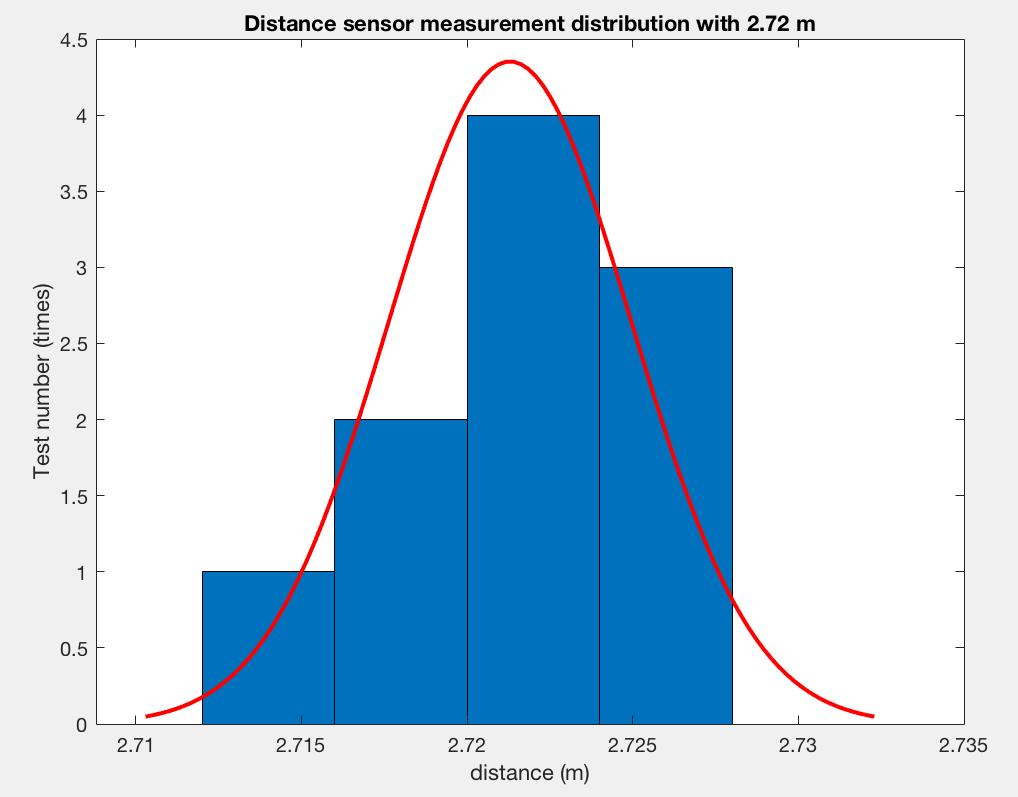
Figure 7: The repeatability distribution of the sensor.

Next, we placed the robot five meters away from the obstacles and measured ten times of the data. We got the average distance value is 0.4451 and the percentage difference is 5.49%, which is still acceptable. Besides, we measured the elapsed time of the sensor is 2.2840e-05 seconds. Once we got these values, we could start designing the program for the robot. The simulator program idea is similar to the real-time obstacle avoidance program. The robot speed is aways constant. We just make the robot turn when the distance is one fifth of the speed. However, we observed that the robot radius is about 0.3 m, and the turning space of its axis is around 0.1 m, so we will need to make the robot backward when the sensor range is less than 0.1 to give the robot room to turn and avoid the obstacle. The program is shown in Figue 8 and the demonstration is shown in Video 5.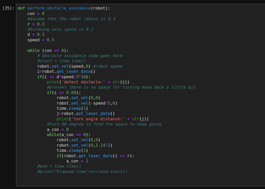

Figure 8: The obstacle avoidance program of the simulator.

Video 5: The demonstration of obstacle avoidance in simulator