Fast Robots: ECE 4960 Lab 6
Objective
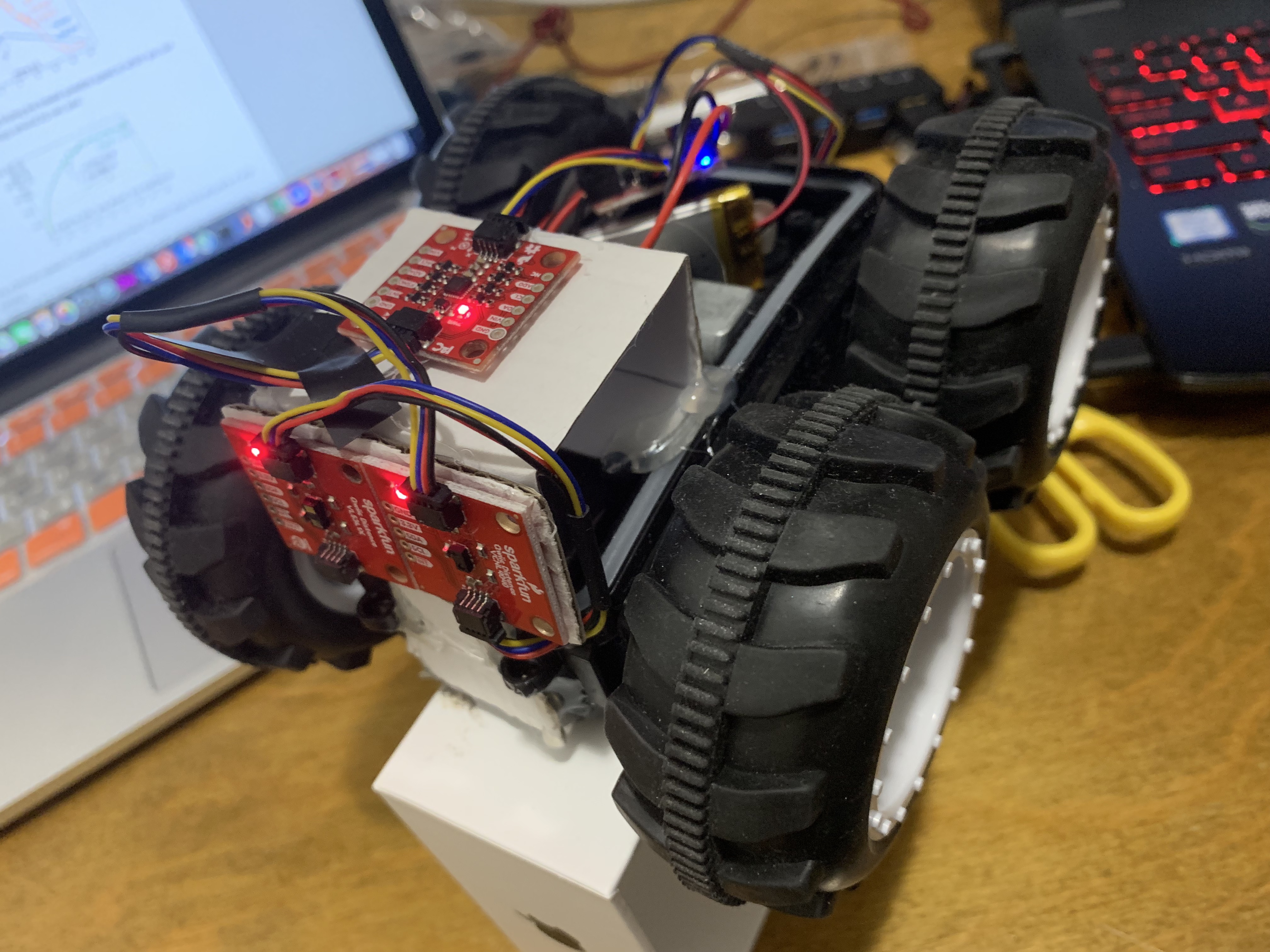
This week, I am going to use the IMU as feedback for the PID controller on the rotational speed. I will use this IMU chip, SparkFun 9DOF IMU Breakout for this lab. I will first test the characteristics of the IMU for its accelerometer, gyroscope, and magnetometer. Then, I am going to design the PID controller based on the data I received and collected data through Bluetooth. Last, I will test the simulation’s plotter tool and observe the difference between the odometry and ground truth pose.Accelerometer
I wired up the IMU with the Artemis board and downloaded the library to run the example program. Before running the code, I checked the I2C address of the board which is “0x69”. The value is matched with the datasheet, so I continued the next process. When I run the program, I could see 10 unique values (3 axes of acceleration, rotational rate, magnetic strength data, and chip’s temperature) on the serial monitor. In order to find the pitch angle and roll angle, I applied these two equations theta = atan(acc_x/acc_z), phi = atan(acc_y/acc_z) on the program. The code is shown in Figure 1. Then, I tried to rotate the IMU in 90, 0, and -90 degrees of the pitch and roll to verify the accuracy of the sensor. The result in Figure 2 shows us the sensor is reliable based on the percentage difference.
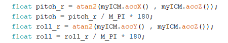
Figure 1: The code of the pitch and roll.
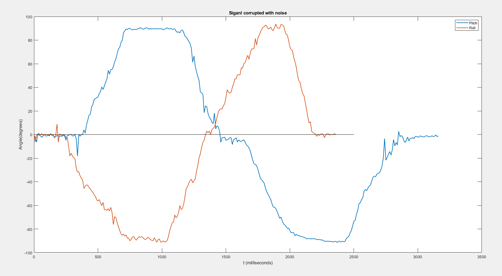
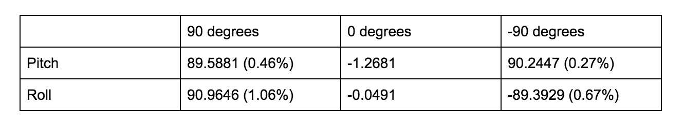
Figure 2: Angle comparison of pitch and roll (left), Angle vs time plot (right).
However, I noticed that if I put the sensor stationary on the table, the data has lots of noise inside, which shows in Figure 3 (top). The average of the number is -6.0002 and the standard deviation is 6.0118, so I did the calibration for the accelerometer. Besides, I tried to tap the IMU that was still, and I found out that there were several peaks occurred, which is shown in Figure 3 (middle), so I use the Fourier transform to see the frequency response of the data. In Figure 3 (bottom), I could see there is a higher peak (red dot) among the data, and the value is 190 Hz.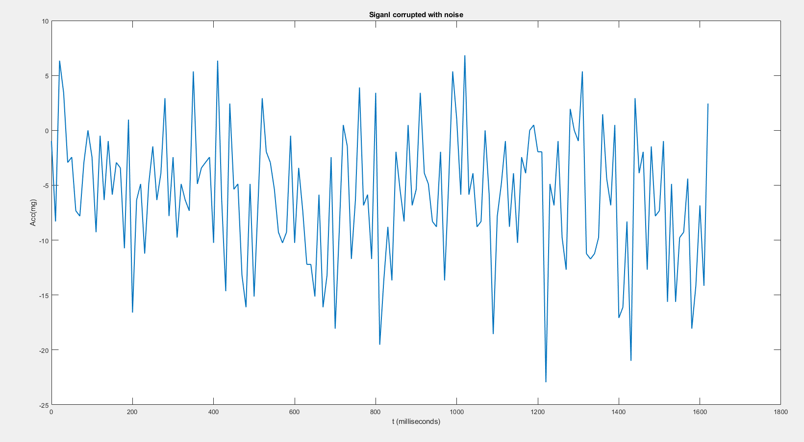
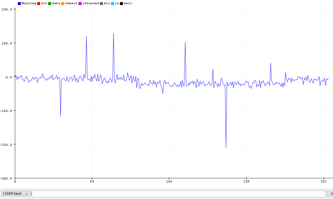
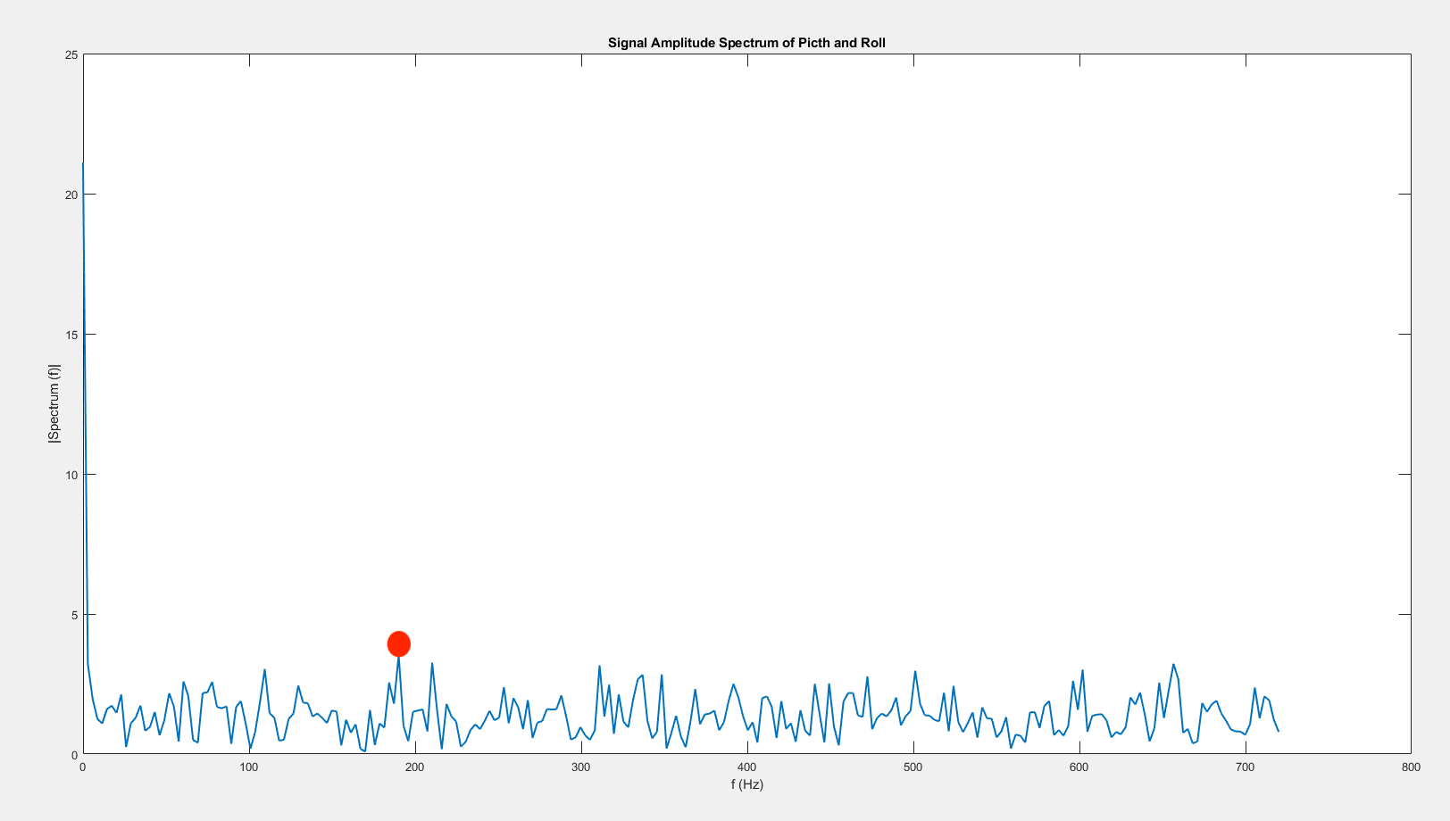
Figure 3: Data with noise (top), Data with tapping (middle), Data applied Fourier transform (bottom).
Therefore, I followed the lecture notes to apply a low-pass filter that shows in Figure 4 (top left) to the data. The sample rate of my program is 100 ms, so the alpha value will be 0.05. I could see the signal is much smoother in Figure 4 (bottom).
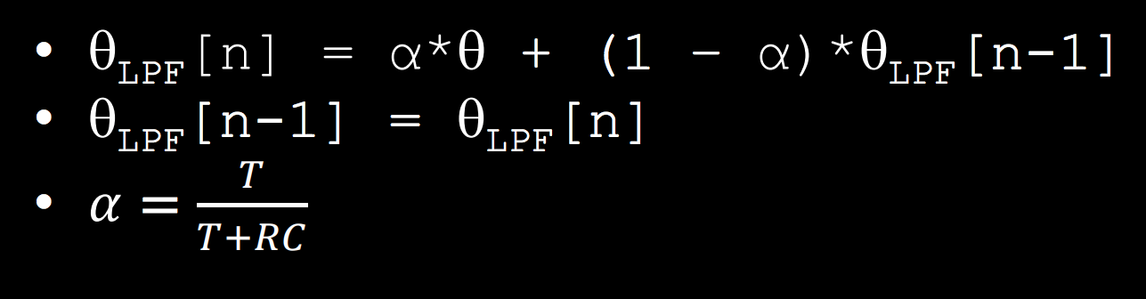
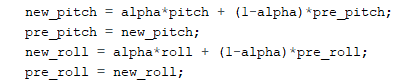
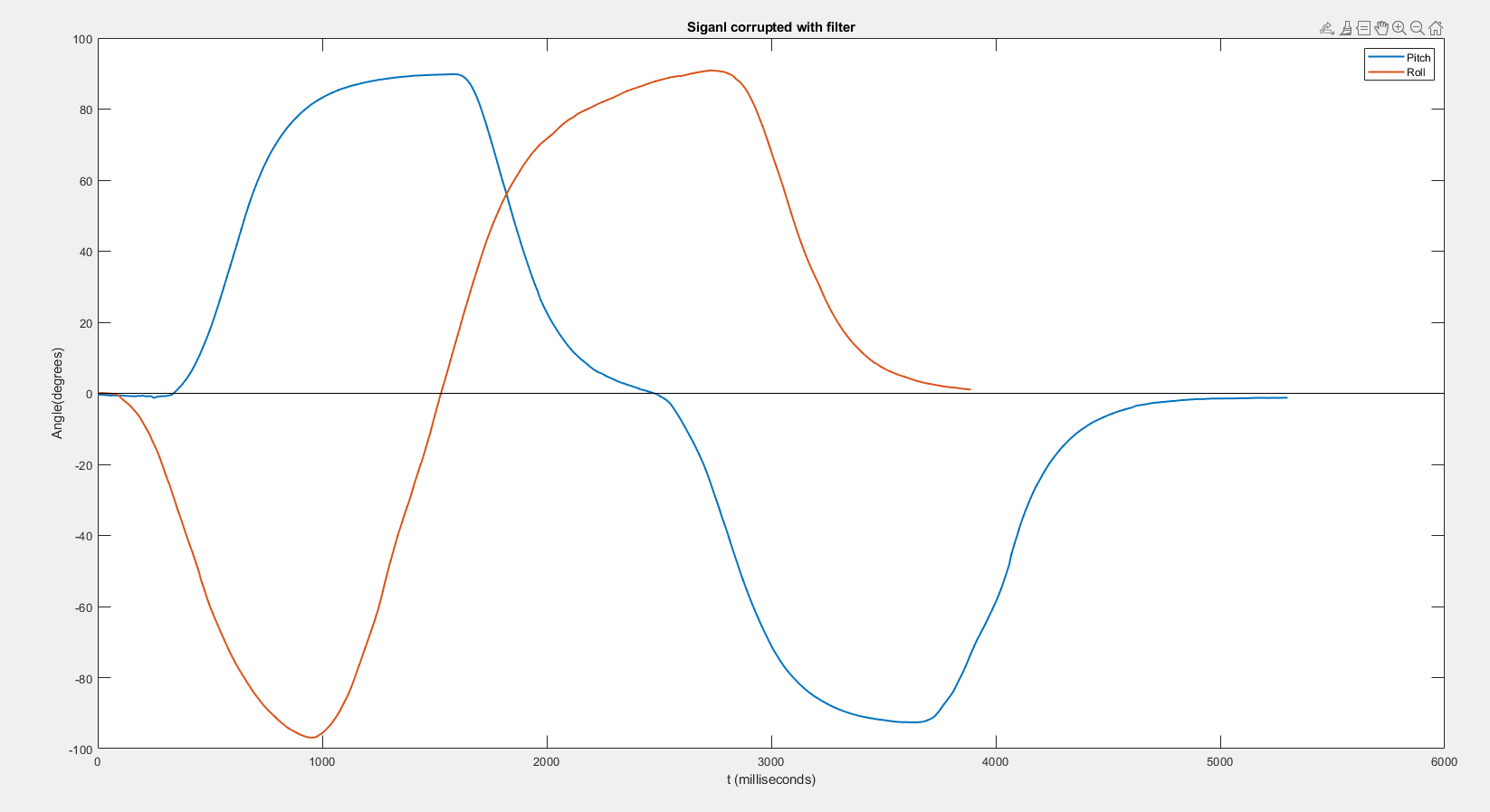
Figure 4: Equation of the low pass filter (top left), LPF code (top right), Pitch and roll with LPF (bottom).
When I compare the data with and without the filter, it can obviously see the effect of the LPF to reduce the noise.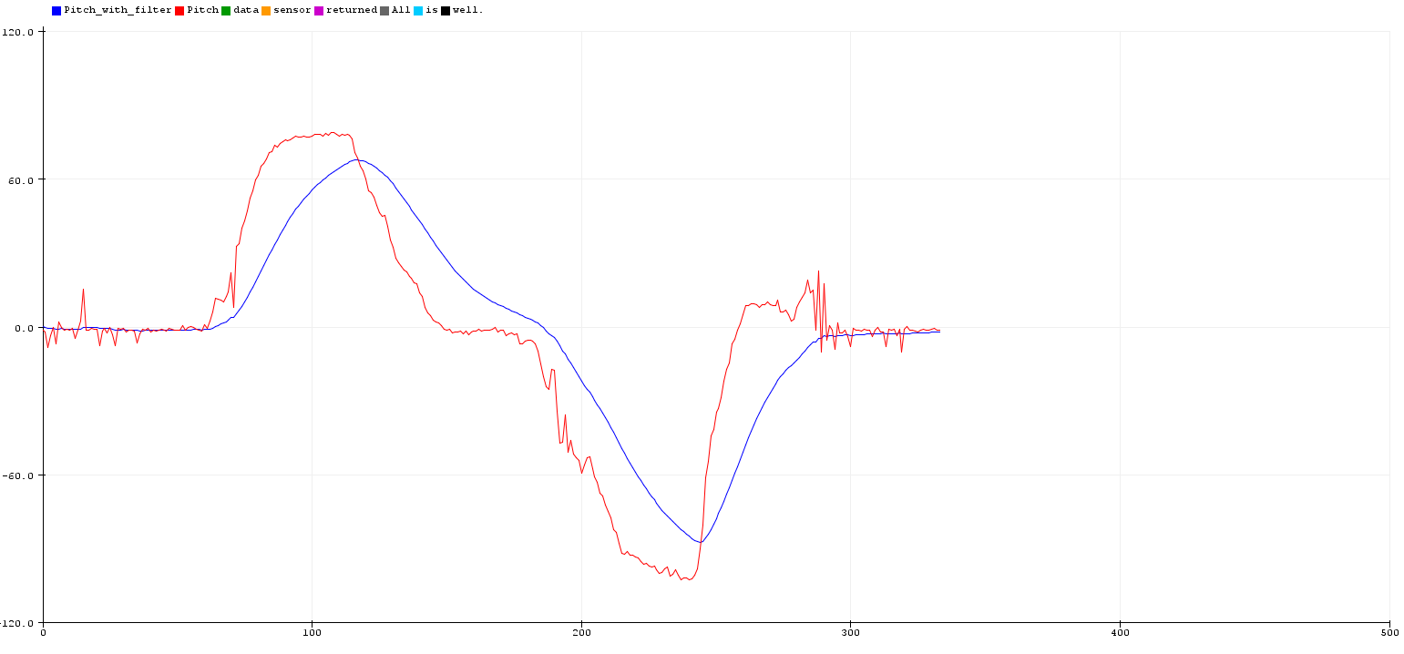
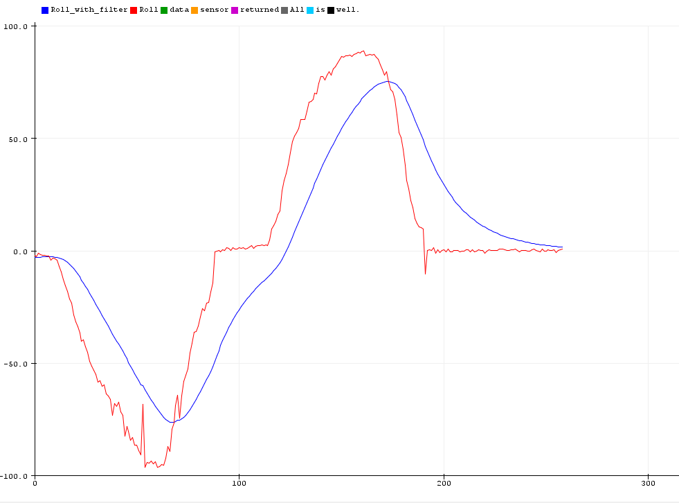
Figure 5: Original pitch and filter pitch (left), Original roll, and filter roll (right).
Gyroscope
Gyroscope is able to measure the rate of angular change [deg/s]. So, I will use the gyroscope to calculate the pitch, roll, and yaw separately by using the equation angle = angle - gyr_reading*dt and compared the result with the filter data from the accelerometer. In Figure 6, the gyroscope data drifts a lot over time and it has a faster response time than the accelerometer. If I decreased the delay time from 100 ms to 10 ms, I see that the gyroscope’s waveform reduces its crest, but it has a similar behavior as the larger delay.
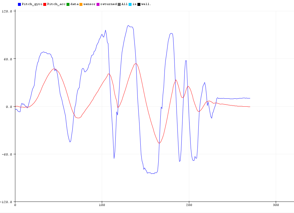
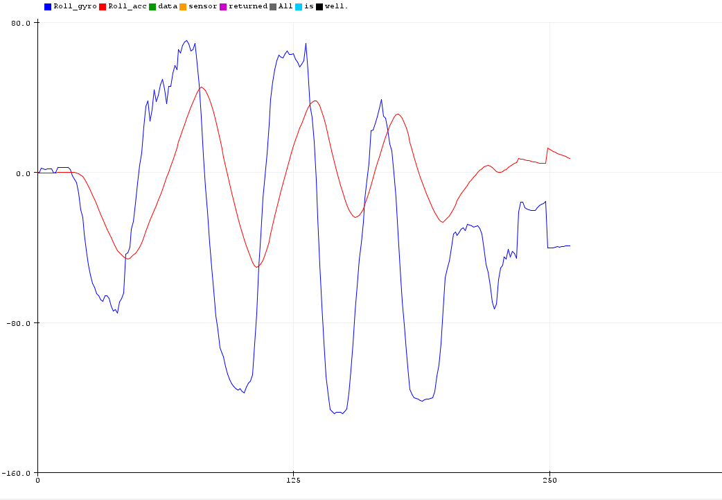
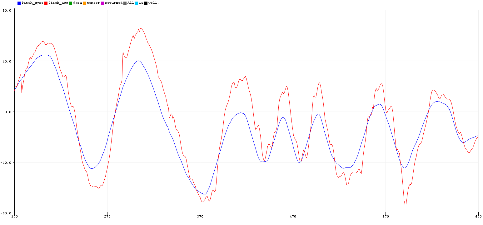
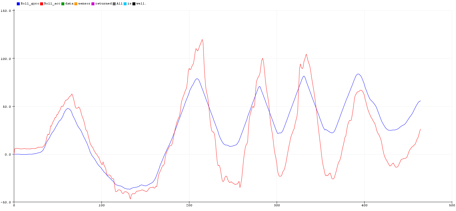
Figure 6: Gyroscope and accelerometer pitch (top left), Gyroscope and accelerometer roll (top right), Gyroscope and accelerometer pitch with delay 10 ms (bottom left), Gyroscope and accelerometer roll with delay 10 ms (bottom right).
Next, in order to reduce the noise from the gyroscope signal, I applied the low-pass filter on the data. The equation is angle = (angle + gyr_reading*dt)*(1-alpha) + acc_reading*alpha . The filter can help reduce the drift but still respond quickly. I used the same alpha value in my program and the results show in Figure 7.
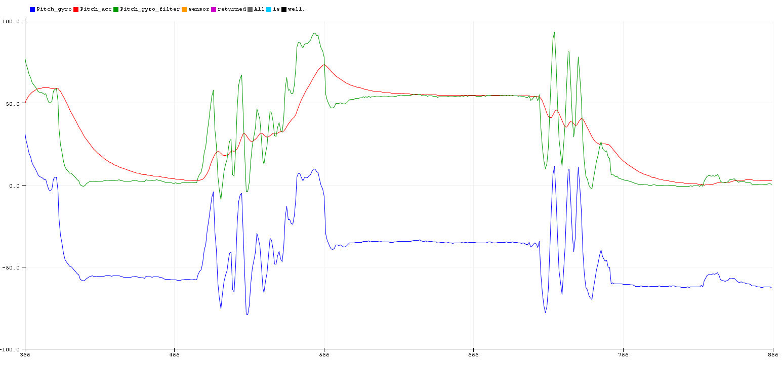
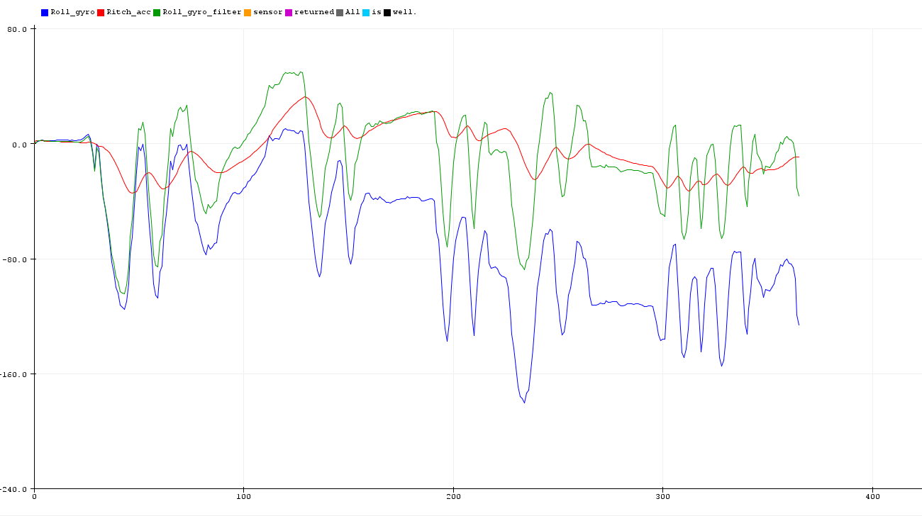
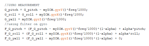
Figure 7: The filtered data (top), the code (bottom).
Magnetometer
Last, I used the equations from class to convert magnetometer data into a yaw angle. I kept the IMU horizontal and rotated it to see the value change. In Figure 8, the yaw value is in the range of [40, -40]. However, the data does not respond quickly and the value does not seem accurate. Also, when I pointed the IMU to the north, the value I got was zero. Hence, I decide to use the gyroscope to calculate the yaw. Although the gyro yaw will keep drifting it has a relatively accurate value to be feedback.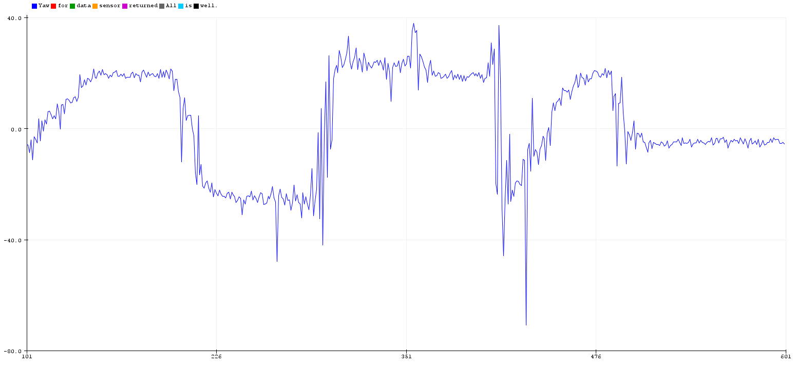

Figure 8: The yaw value from the magnetometer (top), the code (bottom).
PID controller
In the later lab, I will need to apply an algorithm for robot localization and navigation, so it is important to make the robot spin very slowly to make the TOF sensor scan the environment properly. Therefore, we are going to use a proportional–integral–derivative controller (PID controller) and take the rotational yaw value as input/feedback to calculate the output for the motor speed. To achieve the goal, I wrote a program that is able to control the motor to spin in opposite directions at increasing, followed by decreasing, speeds while recording yaw. I made the robot start at 100 and 125 for the left and right motor separately. Also, I set the maximum speed of the robot at 180 (left) and 205 (right) based on the data in lab 5. Moreover, I collected the data through Bluetooth which I set up in lab 2. The result is shown in Figure 9 and the code is distributed in Figure 10. I found that the maximum value of the yaw is around 475 when the speed reaches the maximum.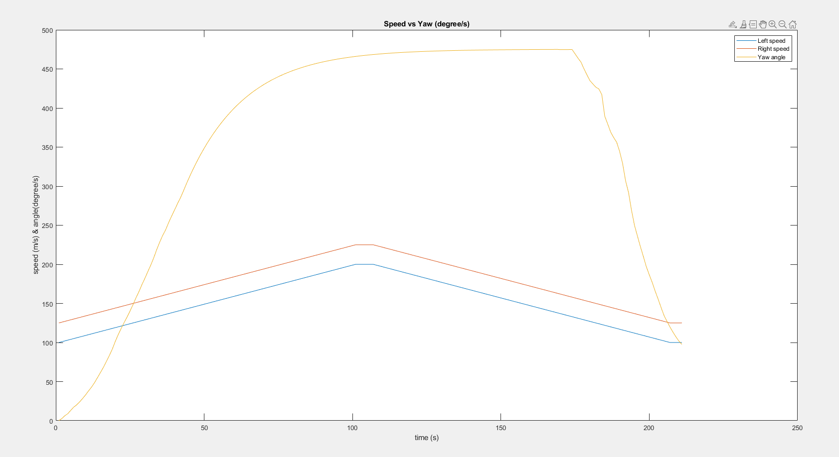
Figure 9: The speed and yaw value diagram.
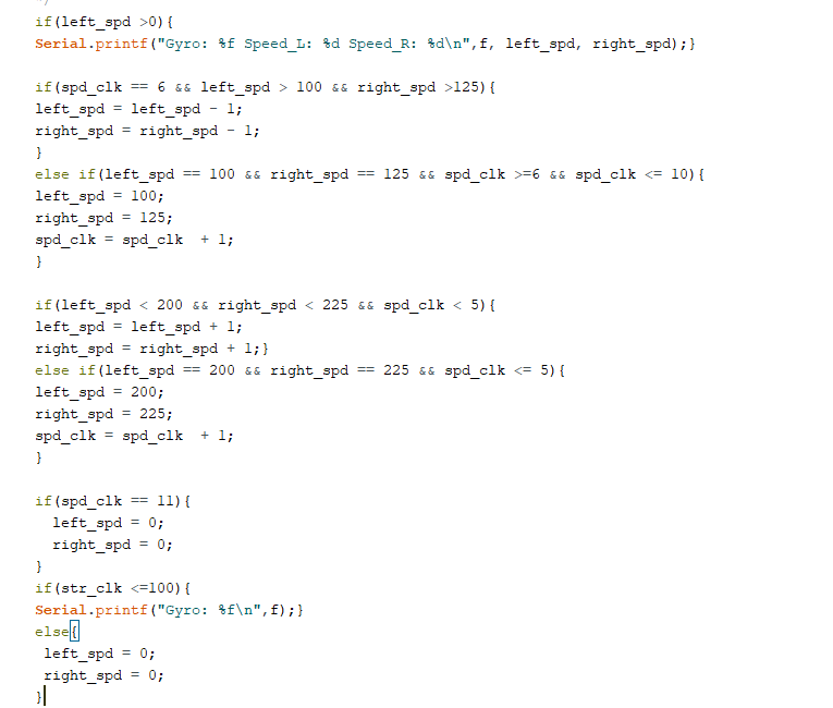
Figure 10: The motor speed control program.
Next, I controlled the motor at a constant speed in order to find the lowest possible speed where the robot can rotate around its own axis. I found that the minimum speed that the robot can rotate around is the left motor at speed 140 and the right motor at speed 165. The yaw value versus speed is shown in Figure 11.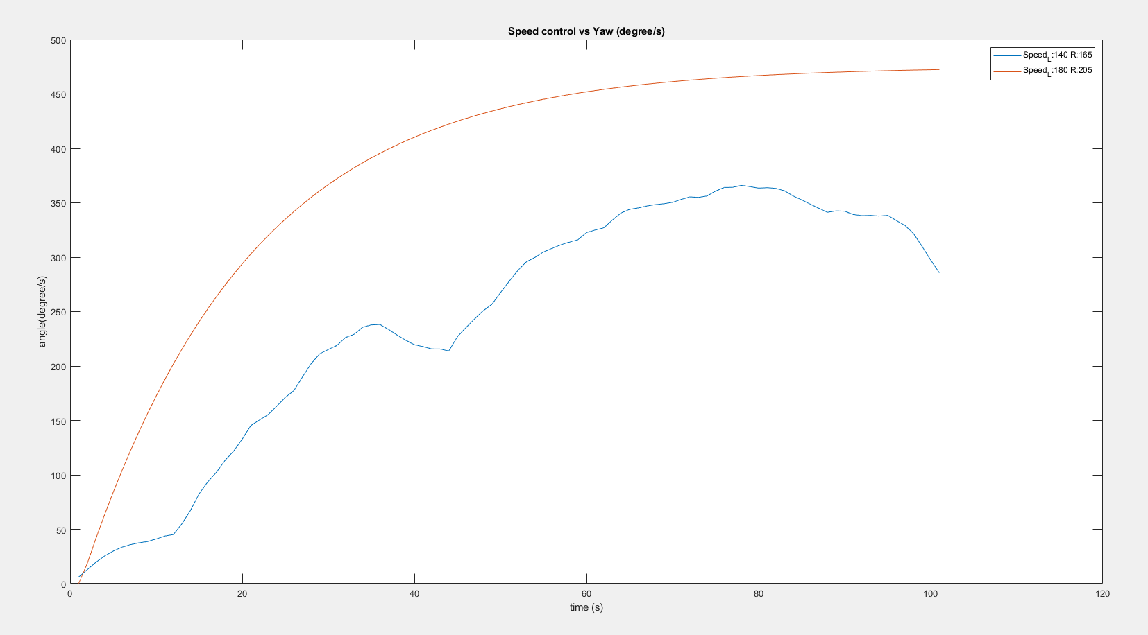
Figure 11: The ramp response at different speeds.
In order to ensure the TOF ranging properly, I made the robot run at the minimum speed and calculated the rotation performance. The robot could rotate 82 degrees per second. If I placed the robot 0.5 meters from a wall pointing straight towards it at the beginning, it will rotate around 2.5 degrees once the Bluetooth collects the first TOF data. Then, I calculated the distance which is 0.5005 meters away from the wall with a delta of 0.0218 meters. If the robot started angled 45 degrees to the wall, the value will be 0.7401 meters away from the wall with a delta of 0.0457 meters. Once I received these data, I started implementing the PID controller. I used the Arduino PID library and took the yaw value as the input in order to find the output as the speed. Based on the yaw value I got in Figure 11, I set the setpoint at 300 and adjust these three parameters (KP, KI, and KD) to observe the different behaviors. I ran five tests with different parameters, which were KP=1, KP=5, KP=20, KP=5 & KI=1, and KP=5&KI=1. The result shows in Figure 12. From the testing, I realized that the speed for the robot is around 120 for the left motor, and the KP=5 produces the best result. However, it is still faster than the loop control in lab 4 which has the minimum speed at 100 for turning. Next, I observed that when the KI increased, the wave became unstable which performed like a sine wave because the integral was in relation not only to the error but also the time where the yaw value has persisted. Video 1 shows the robot rotates with KP = 5 control, and the behavior did match the plot, which rotates fast at first and slows down eventually. However, the robot is sometimes unstable. I considered that when both motors run in different directions, the chip may create an unbalanced current drawn, so one side of the motor will stop at some moment. Furthermore, the speed seems too fast for the TOF to scan and send the data back to the system. Therefore, I will test the PID with only one motor to determine which control I would like to use and observe the difference.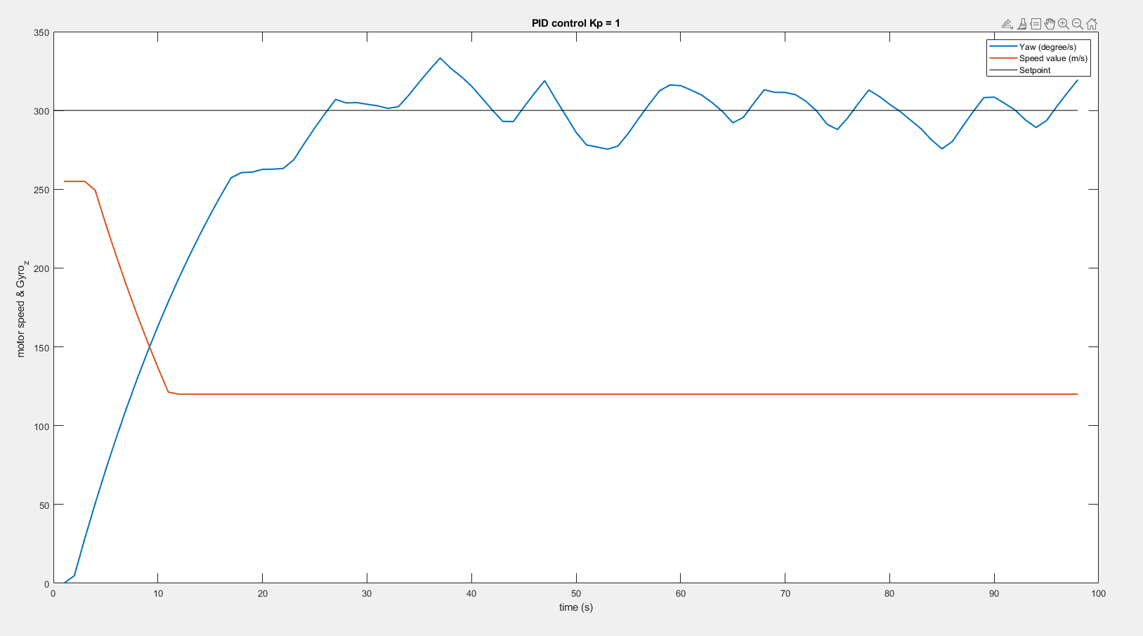
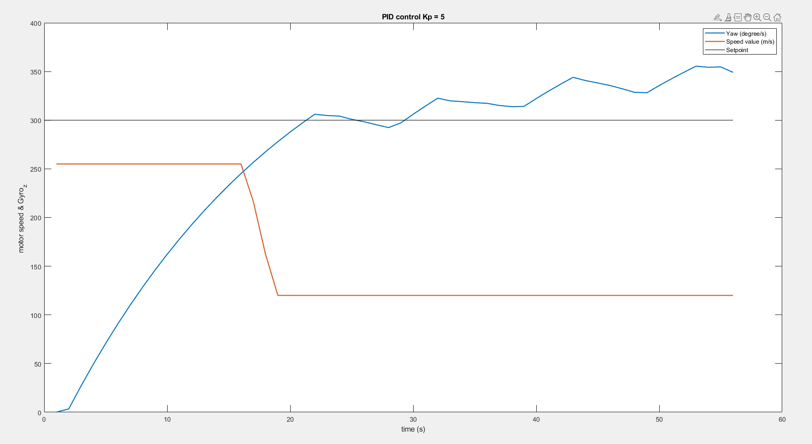
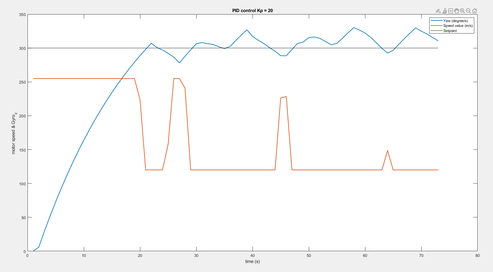
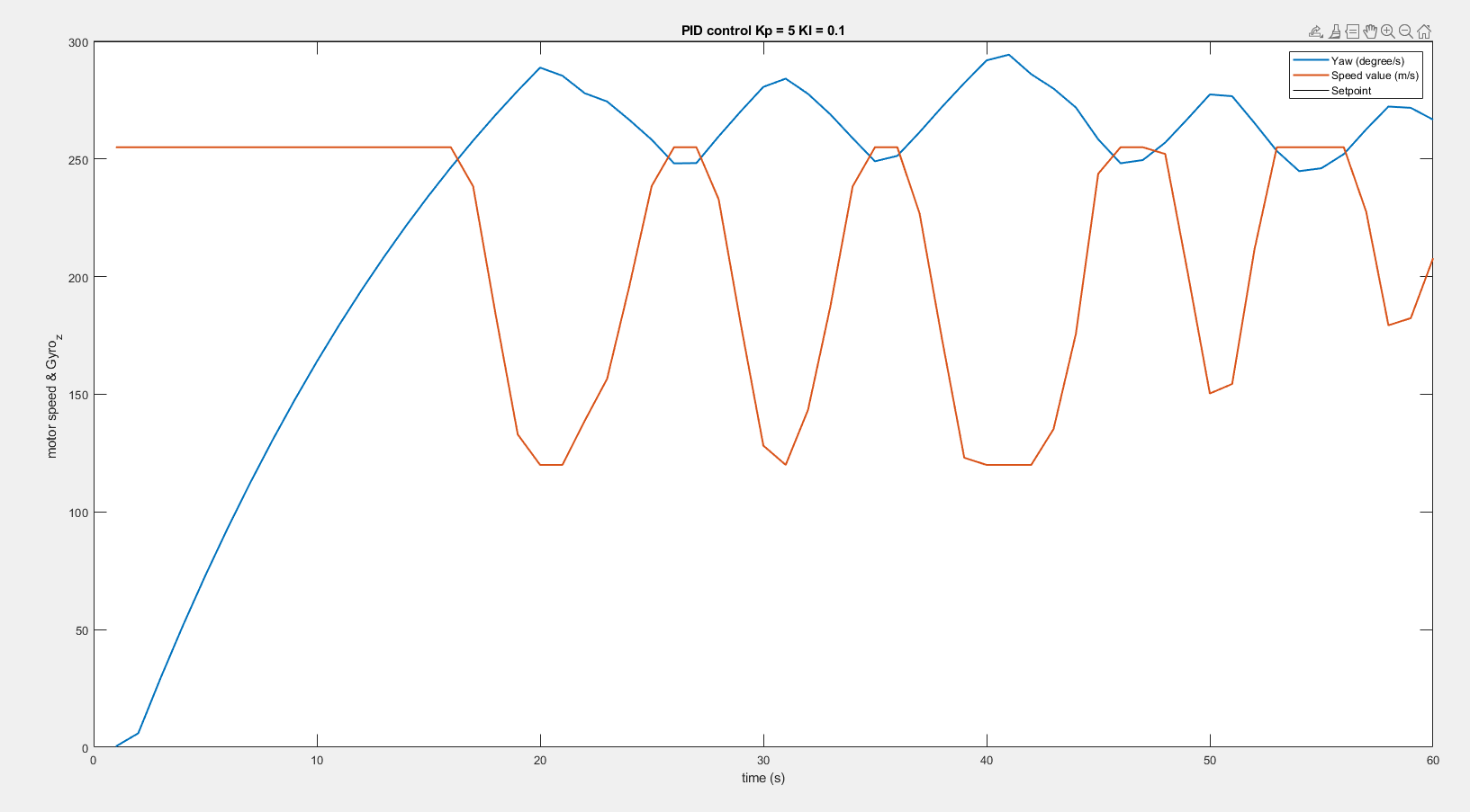

Figure 12: The result with different parameters. The order is KP=1, KP=5, KP=20, KP=5 & KI=1, and KP=5&KI=1.
Video 1: The robot rotates with KP = 5.
The disadvantage of controlling only a single motor is that the robot is hard to spin around its own axis, but it will spin in a wider circle. However, the benefit is that the robot can have a lower speed with a stable system. So, I made the right side motor speed at 10 because the value cannot operate the motor, but it can prevent drifting while the robot is spinning on one side of the motor. The program for the PID control is shown in Figure 13. Then, I started the test with KP = 5 with the setpoint 50 to observe the signal that shows in Figure 14.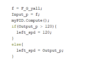
Figure 13: PID program.
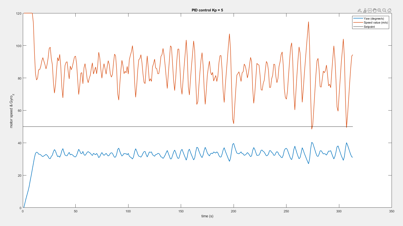
Figure 14: The result with PID control on one motor at KP =5.
I found that the gyroscope value is below the setpoint line, so I tried to use the Ziegler–Nichols method to adjust the parameter. This is a heuristic tuning method. The procedure of the method is to set KI and KD at zero in the beginning. Once KP reaches the ultimate gain where the signal oscillates constantly, we could use the proportion that shows in Figure 15 to adjust the gain. Note: T is the period of the signal wave.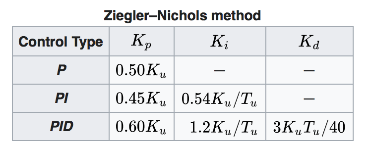
Figure 15: Ziegler–Nichols method table. [1]
I observed the signal wave I plotted, I found the period of my data was 6, so I decided to try the PI control and calculated the KI, which should be 0.9. I realized the gyroscope value was getting closer to the setpoint and it was much smoother but it was still not perfect. Therefore, I calculated the new parameters for the PID control. The parameter’s value is KP = 6, KI = 2, and KD = 4.5. I feel surprised that the signal did match to the setpoint line and the wave had less fluctuation. Besides, the average speed of the motor was 64.43, which was much smaller than I have ever got. The robot will rotate 27 degrees per second. The result is shown in Figure 16.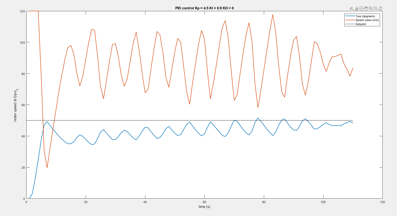
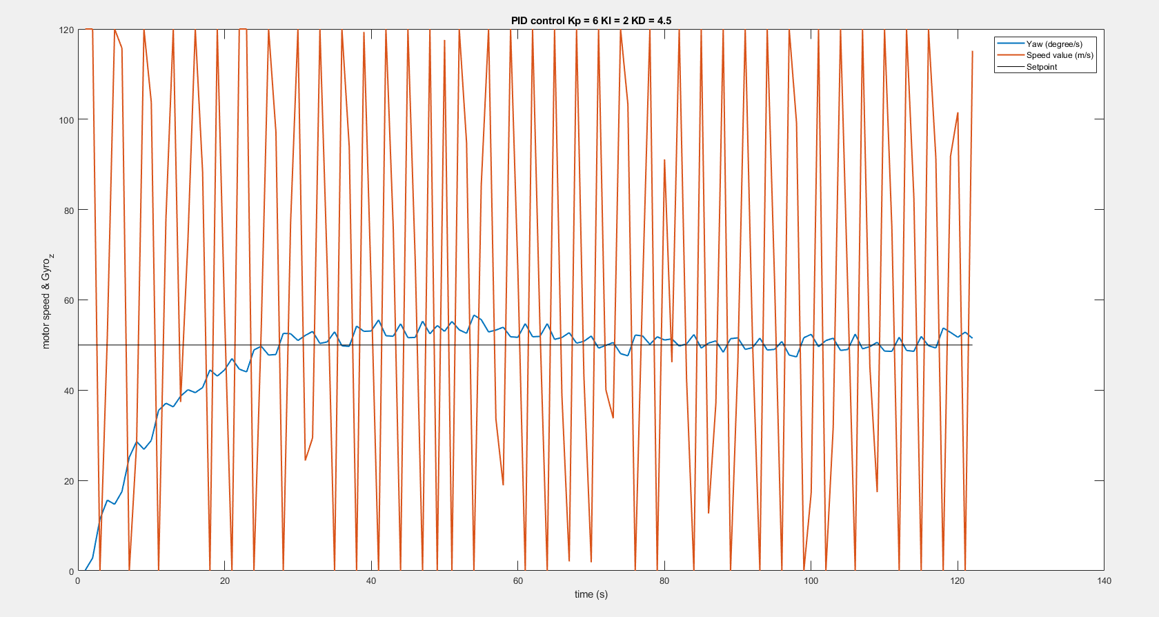
Figure 16: PI control (left), PID control (right).
Last, I have completed the PID controller for my robot, so I would like to try scanning the environment. I placed several obstacles near the robot and the TOP kept ranging for three cycles. The result in Figure 17 shows that the TOF can scan the environment successfully, so I am confident that the robot will be able to map the room properly in lab 7.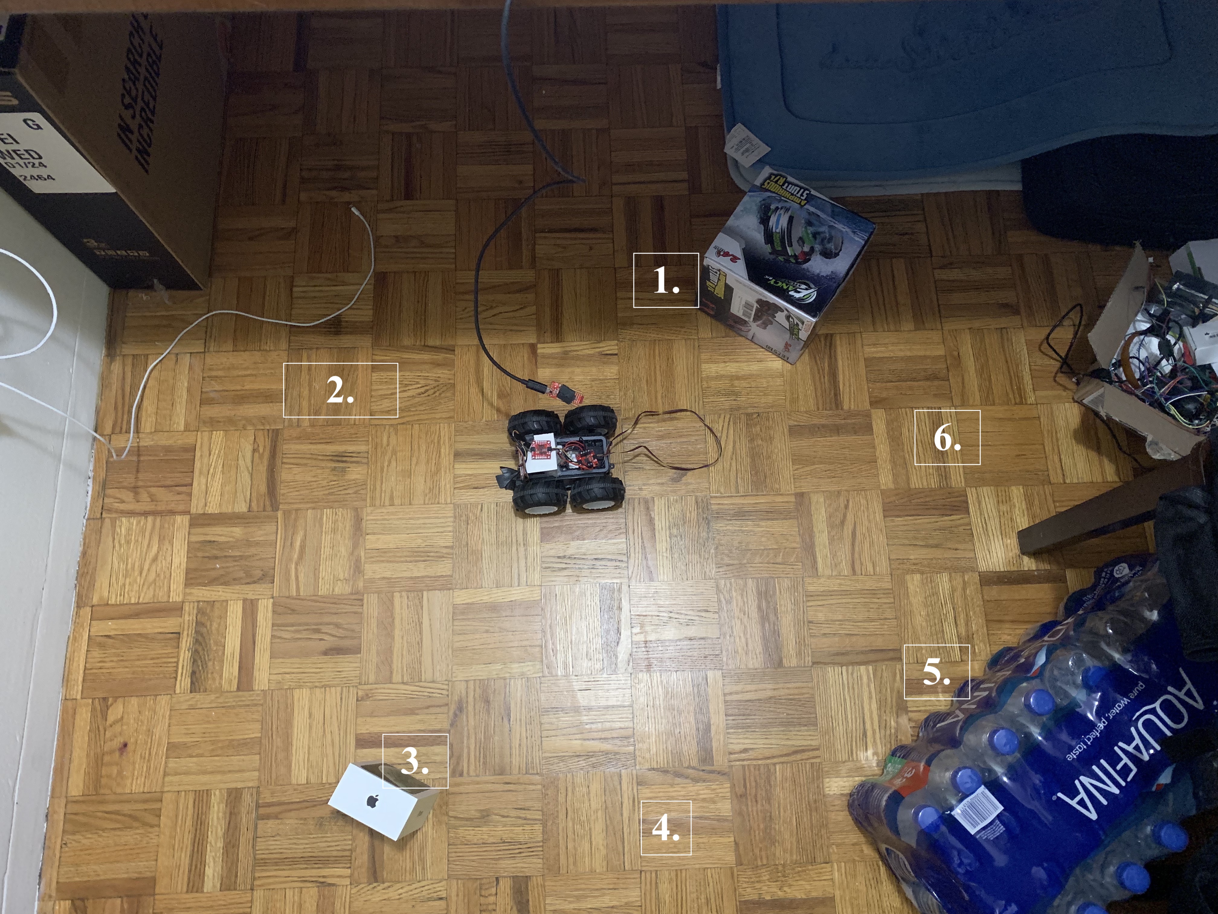
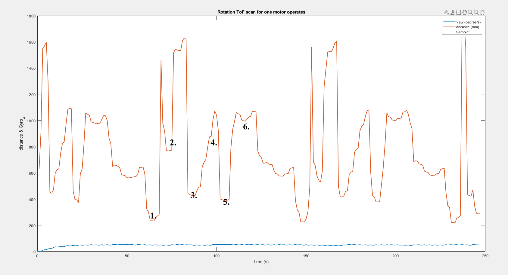
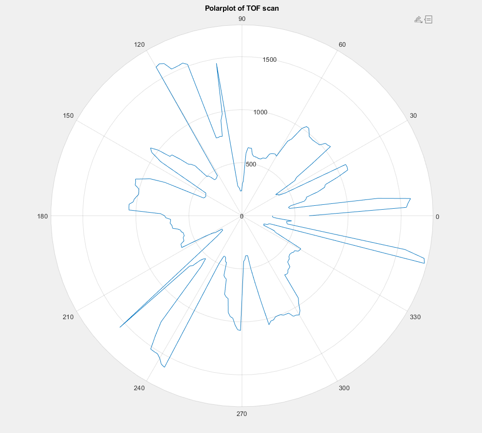
Figure 17: The room environment (left). The result of the TOF ranging (middle). The polar plot (right).
Video 2: The TOF scanning with PID control on one side of the motor.
Simulator
In the simulator section, I am going to run the truth pose estimation and odometry estimation of the virtual robot and compare both data to observe the difference. Odometry is used to estimate the change in position over time, so I expect the odometry trajectory will be similar to the truth pose but it may have an offset without a filter. In the simulator, I sent the data to the plotter every one second. I made the odometry to start at the same point of the truth pose and ran the robot for 25 seconds and 75 seconds to determine whether the time will affect the result. In Figure 18, I realized that the odometry has a similar shape to the truth pose trajectory. However, when the time increases, the offset between the odometry trajectory and the truth pose will increase because the odometry will consider the previous location to predict the next location. If the odometry with noise has a wrong location, then the estimation will become inaccurate when the time increases.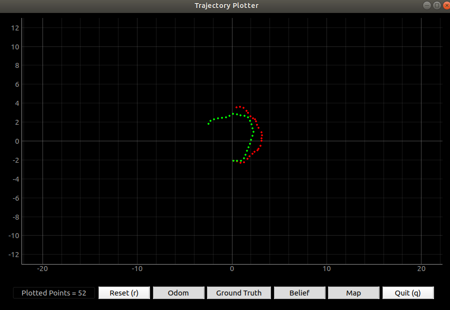
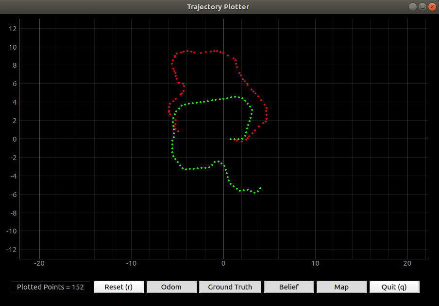
Figure 18: The trajectory of odometry and truth pose with 25 seconds (left) and 75 seconds (right).
Video 3: The plotting progress while the robot is moving.
Besides, I plotted ten points when the robot is stationary and I realized that the truth pose will be fixed but the odometry trajectory will be affected by the noise, which is shown in Figure 19. Therefore, I made the robot move in a straight line (in the x-direction) but at different speeds to discuss whether the speed will affect the noise and the odometry. The x-axes odometry at speed 1 m/s has an average percentage difference of 773.286 % and the y-axes odometry has an average percentage difference of 11.58 %. The x-axes odometry at speed 0.5 m/s has an average percentage difference of 832.28 % and the y-axes odometry has an average percentage difference of 29.41 %. I could see that the noise has a huge influence on the odometry, so I will need to use the Bayes filter to optimize the estimation.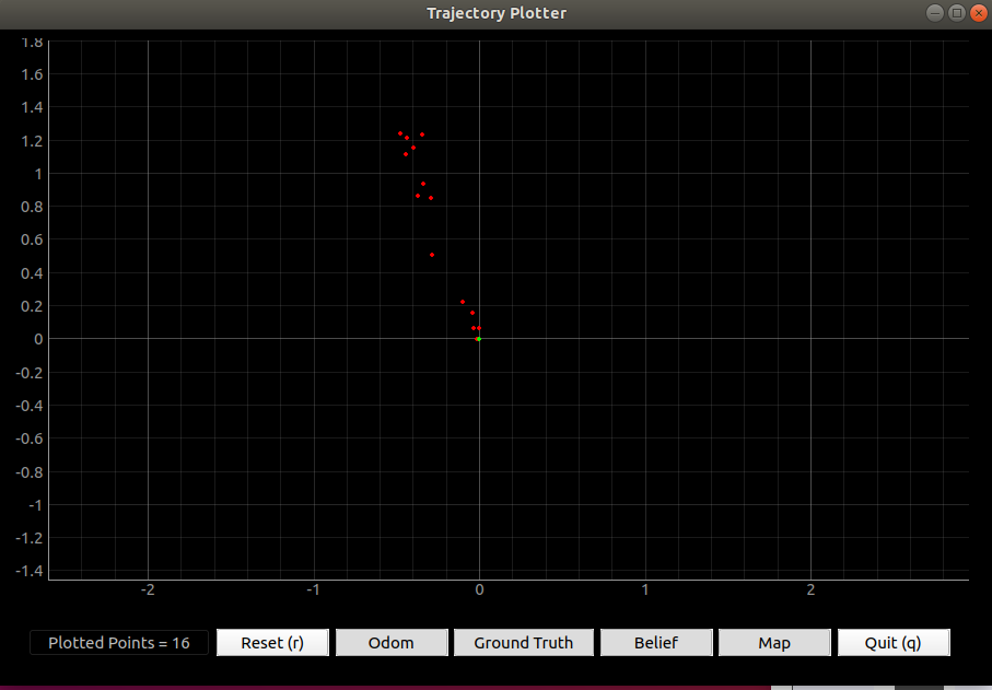
Figure 19: The trajectory of odometry and truth pose when the robot is still.

Figure 20: The simulator plotter code